2 The Shape and Structure of Chemical Data
2.1 Shape of Scientific Data
To understand the successes and failures of machine learning (ML) models, it is instructive to explore how the structure of different datasets shapes the learning capabilities of models. One useful lens for doing so is to consider how complex a system is (i.e., how many variables are needed to describe it) and what fraction of these variables are explicit. One might see the set of variables required to describe a system as the state space. A state space encompasses all possible states of a system, similar to concepts in statistical mechanics (SM).
However, in contrast to many other problems, we often cannot explicitly enumerate all variables and their potential values in relevant chemical systems. Commonly, many of the essential factors describing a system are implicit (“known unknowns” or “unknown unknowns”).
2.1.1 Irreducible Complexity
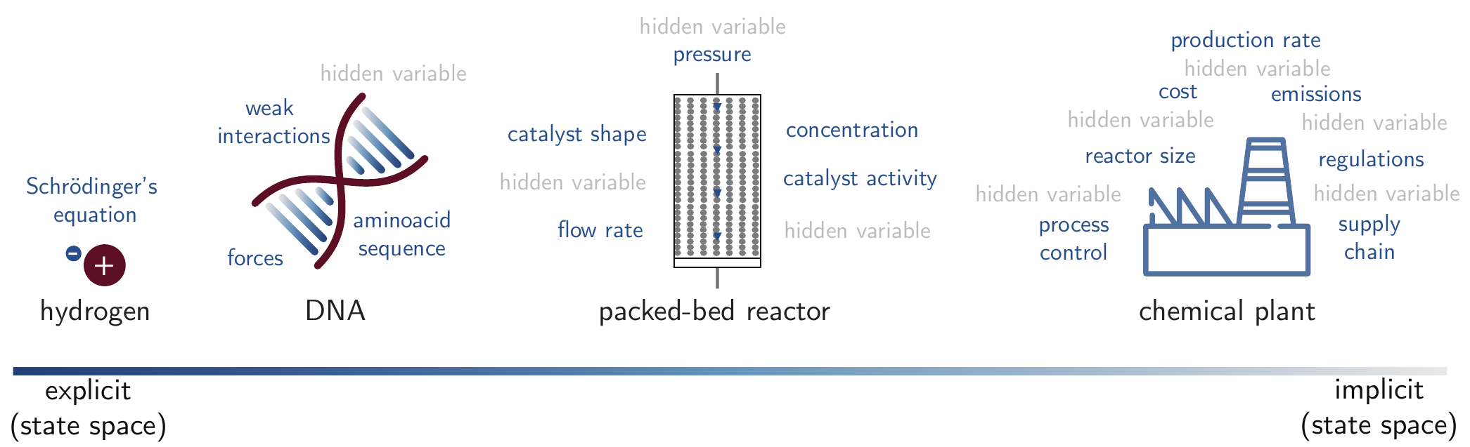
Figure 2.1 illustrates how the state space of chemistry tends to grow more implicit as we move from describing single atoms or small molecules in vacuo, to real-world systems. For instance, we can completely explain almost all observed phenomena for a hydrogen atom using the position (and atomic numbers) of the hydrogen atom via the Schrödinger equation. As we scale up to larger systems such as macromolecular structures or condensed phases, we have to deal with more “known unknowns” and “unknown unknowns”.[Martin (2022)] For example, it is currently impossible to model a full packed-bed reactor at the atomistic scale because the problem scales with the number of parameters that can be tuned. Often, it becomes infeasible to explicitly label all variables and their values. We can describe such complexity as “irreducible”[Pietsch and Wernecke (2017)], in contrast to “emergent” complexity that emerges from systems that can be described with simple equations, such as a double pendulum.
2.1.1.1 Emergent Complexity
In contrast to irreducible complexity, there is a subset of chemical problems for which all relevant parameters can explicitly be listed, but the complexity emerges from the potentially chaotic interactions among them. A well-known example is the Belousov-Zhabotinsky reaction, [Cassani, Monteverde, and Piumetti (2021)] which exhibits oscillations and pattern formation as a result of a complex chemical reaction network. Individual chemical reactions within the network are simple, but their interactions create a dynamic, self-organizing system with properties not seen in the individual components. An example of how fast such a parameter space can grow was provided by Koziarski et al. (2024), who show that a single reaction type and a few hundred molecular building blocks can create tens of thousands of possible solutions. When scaling up to only five reaction types, the exploration of the entire space can become intractable, estimated at approximately \(10^{22}\) solutions.
Knowing the ratio between explicit and implicit parameters helps in selecting the appropriate model architecture. If most of the variance is caused by explicit factors, these can be incorporated as priors or constraints in the model, thereby increasing data efficiency. This strategy can, for instance, be applied in the development of force fields where we know the governing equations and their symmetries, and can use them to enforce such symmetries in the model architecture (as hard restrictions to a family of solutions). [Unke et al. (2021); Musil et al. (2021)] However, when the variance is dominated by implicit factors, such constraints can no longer be formulated, as the governing relationships are not known. In those cases, flexible general-purpose model (GPM)s with soft inductive biases—which guide the model toward preferred solutions without enforcing strict constraints on the solution space[Wilson (2025)]—are more suitable. GPMs such as large language model (LLM)s fall into this category.
2.2 Scale of Chemical Data
Chemistry is an empirical science in which every prediction bears the burden of proof through experimental validation.[Zunger (2019)] However, there is often a mismatch between the realities of a chemistry lab and the datasets on which ML models for chemistry are trained. Much of current data-driven modeling in chemistry focuses on a few large, structured, and highly curated datasets, where most of the variance is explicit (reducible complexity). Such datasets, for example QM9,[Ramakrishnan et al. (2014)] often come from quantum-chemical computations. Experimental chemistry, however, tends to have a significantly higher variance and a greater degree of irreducible complexity. In addition, since data generation is often expensive, datasets are small. Because science is about doing new things for the first time, many datasets also contain at least some unique variables.
Considering the largest chemistry text dataset, ChemPile,[Mirza et al. (2025)] which was produced by curating diverse datasets, we find that the largest dataset is approximately three million times larger than the smallest one (see Table 2.1).
ChemPile[Mirza et al. (2025)] collection. Dominating datasets contribute a large portion of the total token count (a token represents the smallest unit of text that a ML model can process), with the small datasets significantly increasing the diversity.
| Dataset | Token count |
|---|---|
| Three largest ChemPile datasets | |
| NOMAD crystal structures[Scheidgen et al. (2023)] | 5,808,052,794 |
| Open Reaction Database (ORD)[Kearnes et al. (2021)] reaction prediction | 5,347,195,320 |
RDKit molecular features |
5,000,435,822 |
| Three smallest ChemPile datasets | |
| Hydrogen storage materials[HyMARC (n.d.)] | 1,935 |
| List of amino-acids[Alberts (2002)] | 6,000 |
| ORD[Kearnes et al. (2021)] recipe yield prediction | 8,372 |
The prevalence of many small, specialized datasets over large ones is commonly referred to as “the long tail problem”.[Heidorn (2008)]
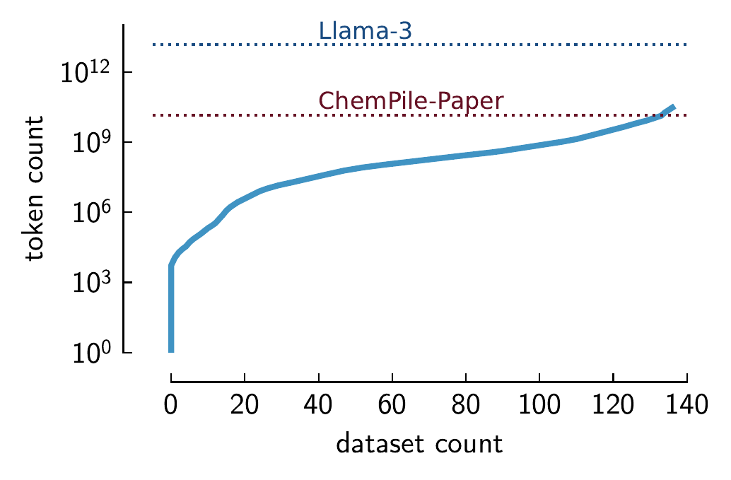
ChemPile tabular datasets (Mirza et al. 2025). We compare the approximate token count for three datasets: Llama-3 training dataset,(Grattafiori et al. 2024) openly available chemistry papers in the ChemPile-Paper dataset, and the ChemPile-LIFT dataset. As can be seen, by aggregating the collection of tabular datasets converted to text format in the ChemPile-LIFT subset, we can achieve the same order of magnitude as the collection of open chemistry papers. However, without smaller datasets, we cannot capture the breadth and complexity of chemistry data, which is essential for training GPMs. The tokenization method for both ChemPile and Llama-3 is provided in the respective papers.
This can be seen in Figure 2.2. We show that while a few datasets are large, the majority of the corpus consists of small but collectively significant and chemically diverse datasets. The actual tail of chemical data is even larger, as Figure 2.2 only shows the distribution for manually curated tabular datasets and not all data actually created in the chemical sciences. Given that every dataset in the long tail has its unique characteristics—it is difficult to leverage this long tail with conventional ML techniques. However, the promise of GPMs is that they can flexibly integrate and jointly model the diversity of small datasets that exist in the chemical sciences.
2.3 Dataset Creation
Training models requires data. For GPMs, the training data must be large and diverse. While raw data can be ingested directly, pre-processed data often works better.
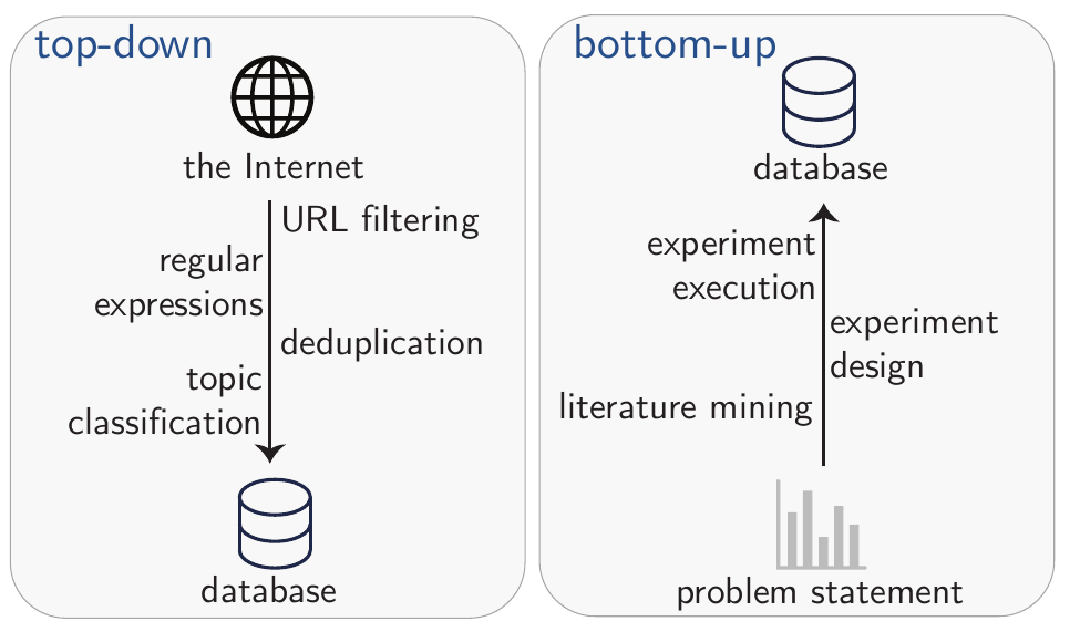
Strategies for compiling data fall into two groups (see Figure 2.3). One can utilize a “top-down” approach where a large and diverse pool of data—e.g., results from web-crawled resources such as CommonCrawl[“Common Crawl” (n.d.)]—is filtered using custom-built procedures (e.g., using regular expressions or classification models). This approach is gaining traction in the development of foundation models such as LLMs.[Penedo et al. (2023); Penedo et al. (2024); Guo et al. (2025)] Alongside large filtered datasets, various data augmentation techniques have further increased the performance of GPMs.[Maini et al. (2024); Pieler et al. (2024)]
Alternatively, one can take a “bottom-up” approach by specifically creating novel datasets for a given problem—an approach which has been very popular in ML for chemistry.
In practice, a combination of both approaches is often used. In most cases, key techniques include filtering and generating synthetic data.
2.3.1 Filtering
While initially the focus was on training on maximally large datasets—enabled by the availability of ever-growing computational resources.[Krizhevsky, Sutskever, and Hinton (2012); Kaplan et al. (2020); Hooker (2020); Dotan and Milli (2019)]—empirical evidence has shown that smaller, higher-quality datasets can lead to better results.[Gunasekar et al. (2023); Marion et al. (2023)] For example, Shao et al. (2024) filtered CommonCrawl for mathematical text using a combination of regular expressions and a custom, iteratively trained classification model. An alternative approach was pursued by Thrush, Potts, and Hashimoto (2024) who introduced a training-free framework. In this method, the pre-training text was chosen by measuring the correlation of each web-domain’s perplexity (a metric that measures how well a language model predicts a sequence of text)—as scored by \(90\) publicly-available LLMs—with downstream benchmark accuracy.
In the chemical domain, ChemPile[Mirza et al. (2025)] is an open-source, pre-training scale dataset that underwent several filtering steps. For example, a large subset of the papers in ChemPile-Paper comes from the Europe PMC dataset.[Consortium (2014)] To filter for chemistry papers, a custom classification model was trained from scratch using topic-labeled data from the CAMEL[Li et al. (2023)] dataset. To evaluate the accuracy of the model, expert-annotated data was used.
2.3.2 Synthetic Data
Instead of only relying on existing datasets, one can also generate synthetic data. Generation of synthetic data is often required to augment scarce real-world data, but can also be used to achieve the desired model behavior (e.g., invariance in image-based models).
These approaches can be grouped into rule-based and generative methods. Rule-based methods apply manually defined transformations—such as rotations and mirroring—to present different representations of the same instance to a model. In contrast, generative augmentation creates new data by applying transformations learned through a ML model.
2.3.2.1 Rule-based Augmentation
The transformations applied for generating new data in rule-based approaches vary depending on the modality (e.g., image, text, or audio). The most common application of rule-based techniques is on images, via image transformations such as distortion, rotation, blurring, or cropping.[Shorten and Khoshgoftaar (2019)] In chemistry, tools like RanDepict[Brinkhaus et al. (2022)] have been used to create enriched datasets of chemical representations. These tools generate drawings of chemical structures that mimic the common illustrations found in scientific literature or even in patents (e.g., by applying image templates from different publishers, or emulating the style of older manuscripts).
Rule-based augmentations can also be applied to text. Early approaches involved operations like random word swapping, random synonym replacement, and random deletions or insertions, which are often labeled “easy augmentation” methods.[Shorten, Khoshgoftaar, and Furht (2021); Wei and Zou (2019)]
In chemistry, text templates have been used.[Xie et al. (2023); Mirza et al. (2025); Jablonka et al. (2024); Van Herck et al. (2025)] Such templates define a sentence structure with configurable fields, which are then filled using structured tabular data. However, it is still unclear how to best construct such templates, as studies have shown that the same data shown in different templates can lead to distinct generalization behavior.[Gonzales et al. (2024)]
We can also apply rule-based augmentation for specific molecular representations (for more details about representations see Section 3.2.1). For example, the same molecule can be represented with multiple different, yet valid simplified molecular input line entry system (SMILES) strings. Bjerrum (2017) used this technique to augment a predictive model, where multiple SMILES strings were mapped to a single property. When averaging the predictions over multiple SMILES strings, at least a \(10\%\) improvement was observed compared to their single SMILES counterparts. Such techniques can be applied to other molecular representations (e.g., International Union of Pure and Applied Chemistry (IUPAC) names or self-referencing embedded strings (SELFIES)), but historically, SMILES has been used more often.[Kimber, Gagnebin, and Volkamer (2021); Born et al. (2023); Arús-Pous et al. (2019); Tetko et al. (2020)]
A broad array of augmentation techniques has been applied to spectral data—from simple noise addition[Ke et al. (2018); Moreno-Barea et al. (2022)] to physics-informed augmentations (e.g., through DFT simulations).[Oviedo et al. (2019); Gao et al. (2020)]
2.3.2.2 Generative Augmentation
In some cases, it is not possible to write down augmentation rules. For instance, it is not obvious how text can be transformed into different styles using rules alone. Recent advances in deep learning have facilitated a more flexible approach to synthetic data generation. [Maini et al. (2024)] A simple technique is to apply contextual augmentation [Kobayashi (2018)], which implies the sampling of synonyms from a probability distribution of a language model (LM). Another technique is “back translation”,[Edunov et al. (2018)] a process in which text is translated to another language and then back into the original language to generate semantically similar variants. While this technique is typically used within the same language,[Lu et al. (2024)] it can also be extended to multilingual setups[Hong et al. (2024)].
Other recent approaches have harnessed auto-formalization[Wu et al. (2022)], a LLM-powered approach that can turn natural-language mathematical proofs into computer-verifiable mathematical languages such as Lean[De Moura et al. (2015)] or Isabelle[Wenzel, Paulson, and Nipkow (2008)]. Such datasets have been utilized to advance mathematical capabilities in LMs.[Xin et al. (2024); Trinh et al. (2024)]
A drawback of generatively augmented data is that its validity is cumbersome to assess at scale, unless it can be verified automatically by a computer program. In addition, it was demonstrated that an increasing ratio of synthetic data can facilitate model collapse.[Kazdan et al. (2024); Shumailov et al. (2024)]
2.4 Future Directions
A primary obstacle in the development of GPMs for chemistry is the immense scale of data required for pre-training, which reaches into the trillions of tokens. This demand is illustrated by models like Llama 3, trained on 15 trillion tokens. Yet the largest open-source chemistry corpus available contains only approximately 75 billion tokens.[Mirza et al. (2025)] Beyond its insufficient volume, this dataset is constrained by restrictive licenses and is not ideally suited for the primary pre-training phase. Furthermore, existing data resources lack documentation of negative or failed experiments and reasoning data related to routine laboratory tasks. The absence of such data impedes the development of robust chemistry problem-solving and planning capabilities in GPMs. This situation stands in contrast to fields like mathematics, where initiatives such as DeepSeek have successfully leveraged large, domain-specific datasets—for instance, 120 billion math tokens—for continual pre-training [Shao et al. (2024)].
Despite the apparent difficulty of amassing diverse data on this scale, we contend that this challenge is accessible through a coordinated community effort.