3 Building Principles of GPMs
3.1 Taxonomy of Foundation Models
In this review, we focus on general-purpose model (GPM)s. Currently, large language model (LLM)s are the most prominent members of the GPM family, but many of the principles discussed here are transferable across different types of GPMs.
In the following, we discuss the inner workings of such models and the process of building them.
3.2 Representations
To interact with any machine, we need to convert the input into numeric values. At its core, all information within a computer is represented as bits (zeros and ones). Bits are grouped into bytes (8 bits), and meaning is assigned to these sequences through encoding schemes like ASCII or UTF-8. Everything—text, a pixel in an image, or even a chemical structure—can be stored as sequences of bytes. For example, “H2O” can be translated into the byte sequence, “H”, “2”, “O”. However, using raw byte sequences for machine learning (ML) presents significant computational inefficiency as representing chemical entities requires long byte sequences, and models would need to learn complex mappings between arbitrary byte patterns and their meanings (as the encoding schemes are not built around chemical principles). Furthermore, handling variable-length sequences can pose additional challenges for models, as they may struggle to perform well on unseen inputs. [Zhou et al. (2023); Baillargeon and Lamontagne (2022)]
A more efficient mapping that is built on top of the underlying byte representation is One-hot encoding (OHE). Instead of working with variable-length byte sequences, we create a fixed vocabulary ({H2O, CO2, HCl}) where each discrete category (in this case, molecule) gets a unique vector: H2O becomes [1, 0, 0], CO2 becomes [0, 1, 0], and so on. This provides unambiguous, computationally manageable representations. As the number of categories grows, one-hot vectors become increasingly long and sparse, making them computationally inefficient—particularly for large vocabularies, i.e., many categories. For example, we need a vocabulary of size 118 to model only the unique elements in the periodic table. Now, imagine the vocabulary required for all unique compounds—assuming one vocabulary element per compound, the size combinatorially explodes. More importantly, while OHE distinguishes molecules or elements, it still treats them as entirely independent. It does not capture any properties of the entity it represents. For example, the ordering of numbers (such as \(4<5\)) or chemical similarities (such as Cl being more similar to Br but less similar to Na) would not be preserved. [Chuang and Keiser (2018)] Embeddings (learned encodings), that we will discuss in Section 3.2.3, solve this through learning dense vector representations.
3.2.1 Common Representations of Molecules and Materials
Before any chemical entity can be converted into a numerical vector—whether through simple OHE or complex learned embeddings—it must first be described in a standardized format (for example, if we are working with materials, it should be able to encode all materials), which is then mapped to encodings.
For complex entities like molecules, materials, and reactions, this choice of what fundamental units to represent (“should we include only atomic numbers?”, “Should we include something about the coordinates?”, etc.) is thus among the most consequential decisions in building a model. It determines the inductive biases—the set of assumptions that guide learning algorithms toward specific patterns over others.[Huang and Lilienfeld (2016)] The landscape of chemical representations reflects different answers to this question, each making distinct trade-offs between simplicity, expressiveness, and computational efficiency (see Table 3.1).
| Representation | Encoded information | Description | Example |
|---|---|---|---|
| Elemental composition | Stoichiometry | Always available, but non-unique. | C9H8O4 |
| International Union of Pure and Applied Chemistry (IUPAC) name | Stoichiometry, bonding, geometry | Universally understood, systematic nomenclature, unmanageable for large molecules, and lacks detailed 3D information. | 2-acetyloxybenzoic acid |
| simplified molecular input line entry system (SMILES) [Weininger (1988)] | Stoichiometry, bonding | Massive public corpora and tooling support, however, there are several valid strings per molecule, and it does not contain spatial information. | CC(=O)OC1=CC=CC=C1C(=O)O, O=C(O)c1ccccc1OC(C)=O, etc. |
| self-referencing embedded strings (SELFIES) [Krenn et al. (2020)]; [Cheng et al. (2023)] | Stoichiometry, bonding | 100% syntactic and semantic validity by construction, including meaningful grouping. | [C][C][=Branch1][C][=O][O][C][=C][C][=C][C][=C][Ring1][=Branch1][C][=Branch1][C][=O][O] |
| international chemical identifier (InChI) | Stoichiometry, bonding | Canonical one-to-one identifier; encodes stereochemistry layers. | InChI=1S/C9H8O4/c1-6(10)13-8-5-3-2-4-7(8)9(11)12/h2-5H,1H3,(H,11,12) |
| Graphs | Stoichiometry, bonding, geometry | Strong inductive bias that works with graph neural network (GNN)s. Symmetry-equivariant variants available. Long-range interactions are implicit. | 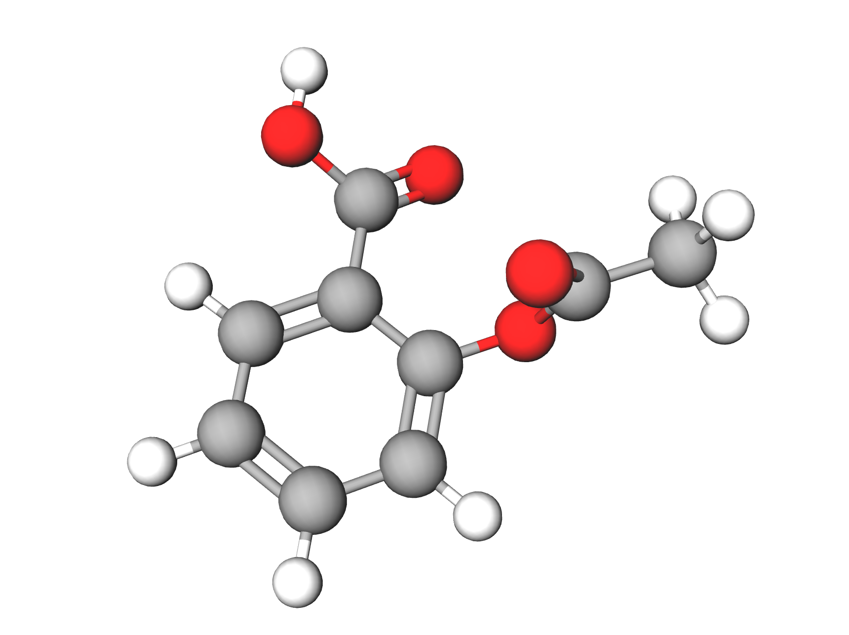 |
| xyz representation | Stoichiometry, geometry | Exact spatial detail. It is high dimensional, and orientation alignment is needed. | 1.2333 0.5540 0.7792 O -0.6952 -2.7148 -0.7502 O 0.7958 -2.1843 0.8685 O 1.7813 0.8105 -1.4821 O -0.0857 0.6088 0.4403 C … |
| Multimodal | Stoichiometry, bonding, geometry, symmetry, periodicity, coarse graining | Combines complementary signals; boosts robustness and coverage. It is hard to implement, the complexity scales with the amount of representations, some modalities are data-scarce, and the information encoded totally depends on the modalities included. | 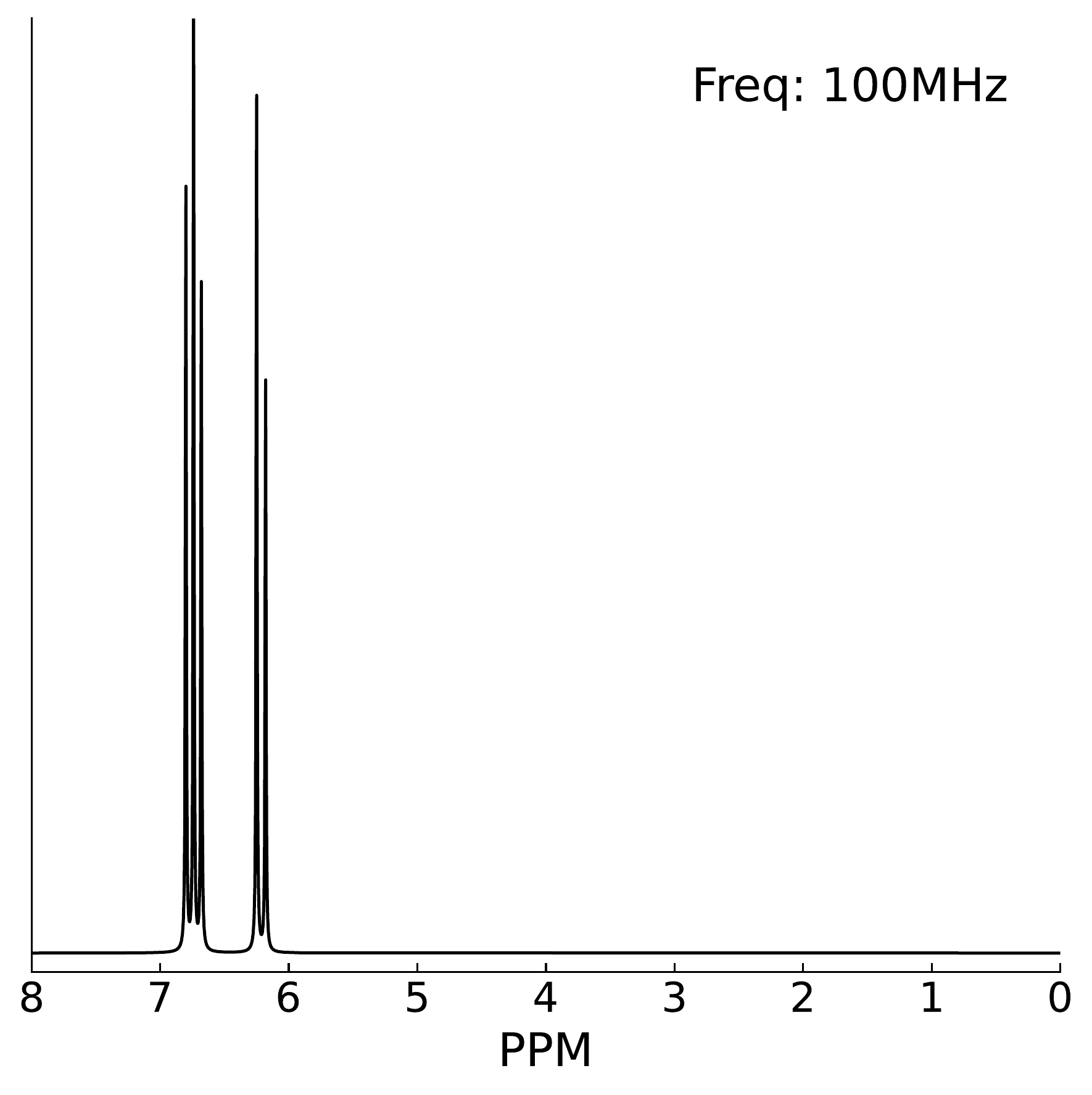 |
| crystallographic information file (CIF) [Hall, Allen, and Brown (1991)] | Stoichiometry, bonding, geometry, periodicity | Standardized and widely supported, however, it carries heterogeneous keyword sets and parser overhead | data_Si _symmetry_space_group_name_H-M ’P 1’ _cell_length_a 3.85 …_cell_angle_alpha 60.0 …_symmetry_Int_Tables_number 1 _chemical_formula_structural Si _chemical_formula_sum Si2 _cell_volume 40.33 _cell_formula_units_Z 2 loop_ _symmetry_equiv_pos_site_id _symmetry_equiv_pos_as_xyz 1 ’x, y, z’ loop_ _atom_type_symbol _atom_type_oxidation_number Si0+ 0.0loop_ _atom_site_type_symbol _atom_site_label _atom_site_symmetry_multiplicity _atom_site_fract_x …_atom_site_occupancy Si0+ Si0 1 0.75 0.75 0.75 1.0 Si0+ Si1 1 0.0 0.0 0.0 1.0 |
| Condensed CIF [Gruver et al. (2024); Antunes, Butler, and Grau-Crespo (2024)] | Stoichiometry, geometry, symmetry, periodicity | Good for crystal generation tasks. It omits occupancies and defects, custom tooling is needed, and only works for crystals | 3.8 3.8 3.8 59 59 59 Si0+ 0.75 0.75 0.75 Si0+ 0.00 0.00 0.00 |
| simplified line-input crystal-encoding system (SLICES) [Xiao et al. (2023)] | Stoichiometry, bonding, periodicity | Invertible, symmetry-invariant and compact for general crystals. However, it carries ambiguity for disordered sites | Si Si 0 1 + + + 0 1 + + o 0 1 + o + 0 1 o + + |
| local-environment (Local-Env) [Alampara, Miret, and Jablonka (2024)] | Stoichiometry, bonding, symmetry, coarse graining | Treats each coordination polyhedron as a “molecule”, it is transferable and compact; but it ignores long-range order and its reconstruction requires post-processing | R-3m Si (2c) [Si][Si]([Si])[Si] |
| Natural-language description [Ganose and Jain (2019)] | Stoichiometry, bonding, geometry, symmetry, periodicity, coarse graining | It is human-readable and tokenizable in a meaningful way by pretrained LLMs. However, trying to encode all the information can lead to verbose, ambiguous descriptions. | “Silicon crystallizes in the diamond-cubic structure, a lattice you can picture as two face-centred-cubic frameworks gently interpenetrating…” |
A common strategy is to represent chemical information as a sequence of characters. This allows us to leverage architectures initially designed for natural language. This approach has found success in language modeling for predicting protein structures and functions, where the amino acid sequence, the foundation of a protein’s structure and function, is easily represented as text.[Rives et al. (2021); Elnaggar et al. (2022); Ruffolo and Madani (2024)] The most prevalent string representation for molecules in chemistry is SMILES[Weininger (1988)]. SMILES strings provide a linear textual representation of a molecular graph, including information about atoms, bonds, and rings. However, SMILES representations have limitations. The same molecule can be represented through multiple valid SMILES strings (so-called non-canonical representations). Although the existence of non-canonical representations enables data augmentation (see Section 2.3.2), it can also confuse models because the same molecule would have different encodings, each one originating from a different SMILES string. In addition, SMILES imposes a relatively weak inductive bias; the model must still learn the rules of valence and bonding from the grammar of these character sequences. Moreover, SMILES does not preserve locality: structural motifs that are directly bonded or physically close to each other in a molecule can be very far apart in the SMILES representation.
A limitation of SMILES is that not every SMILES string corresponds to a valid molecule. A more robust alternative is SELFIES[Krenn et al. (2020); Cheng et al. (2023)], where every SELFIES corresponds to a valid molecule, providing a stronger bias towards chemically plausible structures (chemical validity biases). The InChI is another standardized string representation. Unlike SMILES, InChI strings, as identifiers, are canonical—each molecule has exactly one InChI representation. This eliminates ambiguity, but comes at the cost of human readability and increased string length.
In the realm of materials, no natural representation has emerged. Previous work has indicated that for certain phenomena (e.g., when all structures in a dataset are in the ground state), composition might implicitly encode geometric information [Tian et al. (2022); Jha et al. (2018); A. Y.-T. Wang et al. (2021)] and composition alone can be predictive of various material properties. Thus, it is a widely chosen method to represent materials, depending on the task. When structural information is available, CIFs, initially proposed as a standard way to archive structural data in crystallography [Hall, Allen, and Brown (1991)], is now a widely used representation. [Gruver et al. (2024); Antunes, Butler, and Grau-Crespo (2024)] proposed a condensed version of CIFs, which includes only the parameters necessary for building the crystal structure in a crystal generation application. Ganose and Jain (2019) aimed to create human-readable descriptions by proposing a tool to generate natural-language descriptions of crystal structures automatically. For specific material classes, such as metal-organic framework (MOF)s, specialized representations like MOFid [Bucior et al. (2019)] have been developed.
As an alternative to strings, we can represent molecules and materials as graphs. Here, we directly encode atoms (nodes) and bonds (edges). This representation introduces strong locality biases that explicitly inform the model about atomic connectivity, so the model does not need to learn this fundamental principle from scratch. Symmetry has been incorporated into many of the best-performing graph-based approaches by designing symmetry-constrained representations [Langer, Goeßmann, and Rupp (2022); Musil et al. (2021)] and architectures [Satorras, Hoogeboom, and Welling (2021); Batzner et al. (2022)].
Ultimately, weaker inductive biases (like text) offer greater flexibility and can capture unexpected patterns, but may require more data to learn the fundamental rules. The successful design of inductive biases requires balancing domain knowledge with learning flexibility. Stricter inductive biases (like graphs) incorporate more domain knowledge, leading to greater data efficiency but potentially limiting the model’s ability to discover patterns that contradict our initial assumptions.
Beyond choosing a single optimal representation, GPMs allows for the simultaneous use of multiple representations. A chemical entity can be described not only by its textual SMILES string or its connectivity graph, but also by its experimental or simulated spectra (e.g., NMR, infrared spectroscopy (IR)), or even a microscopy image. Each of these modalities provides a complementary layer of information. A more detailed section on using multiple representations is presented in Section 3.9.1.
3.2.2 Tokenization
Once we have chosen a representation format—whether SMILES strings, CIF files, or chemical formulas—we face another fundamental question: How does a model process these variable-length sequences of characters? One might imagine creating a unique identifier or encoding for every single molecule or string. It is impractical to have a dictionary entry for every sentence in a language due to the similar scaling problems of OHE.
Consider the molecule with the SMILES string CN1C=NC=C1C(=O). We could break down the representation in several ways: as individual characters (C, N, 1, C, =, etc.), as atom-bond pairs (CN, C=, NC), or as fragments (CN1, C=NC, etc.). Each choice creates a different “language” for the model to learn, with distinct computational and learning implications (see example Note 3.1).
This is where tokenization becomes essential. It is the strategy of breaking down a complex representation (like a SMILES string) into a sequence of discrete, manageable units called tokens. The core idea is to find a set of common, reusable building blocks. Instead of learning about countless individual molecules, the model knows a much smaller, finite vocabulary of tokens. By learning an encoding for each token, the model gains the ability to understand and construct representations for an immense number of molecules—including those it has never seen before—by combining the meanings of their constituent parts. This compositional approach enables generalization.
Tokenization strategies for caffeine SMILES (CN1C=NC2=C1C(=O)N(C(=O)N2C)C):
- Character-level: [
C,N,1,C,=,N,C,2,=,C,1,C,(,=,O,),N,(, …] - Chemical fragments: [
CN1C=NC2=C1,C(=O),N(,C(=O), …]
The choice affects what the model learns. Character-level requires learning chemical rules from scratch, while fragment-level embeds chemical knowledge but needs a larger vocabulary.
The concept of tokenization, or defining the fundamental units of input, extends beyond string-based representations. In images, it could be patches of images. In graph-based models, the analogous decision is how to define the features for each node (atom) and edge (bond). Should a node represent an atomic number (a simple “token”), or should it be a more complex sub-structure like a structural motif[Bouritsas et al. (2022)] (a richer “token”)? This choice determines the level of chemical knowledge initially provided to the model. Ultimately, the tokenization strategy defines the elementary units for which the model will learn embeddings, setting the stage for learning the context-aware representations discussed next.
3.2.3 Embeddings
Through training, models can learn to map discrete inputs into continuous spaces where similar items have meaningful relationships (for example, similar items cluster in this continuous space). In the simplest approach, they can be created by training models (so-called Word2Vec models) that take one-hot encoded inputs and predict the probability of words in the context.[Mikolov, Chen, et al. (2013); Mikolov, Sutskever, et al. (2013); Tshitoyan et al. (2019)] Embeddings are powerful because they learn relationships between entities, allowing for the efficient compression of data and the uncovering of hidden patterns that would otherwise be invisible in the raw data.
The advent of GPMs has further underscored the usefulness of high-quality embeddings. These models, trained on vast amounts of chemical data, learn to create powerful, generalizable embeddings that can be adapted to a wide range of downstream tasks, from property prediction (see Section 6.1) to molecular generation (see Section 6.2). In the following sections, we describe the process of generating, refining, and using these embeddings through training and different architectures.
3.3 General Training Workflow
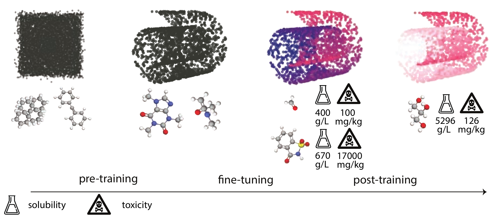
The entire training process of a GPM typically contains multiple steps that can be divided into two broad groups (see Figure 3.1). [Howard and Ruder (2018)] The first step is pre-training, which is usually done in a self-supervised manner and focuses on learning a data distribution—the underlying set of rules and patterns that make up the data. Imagine all possible arrangements of atoms, both real and unfeasible. The data distribution describes which molecules are “likely” (stable, following chemical rules) and which are “unlikely” or “impossible” (random assortments of atoms).
In pre-training the model learns the “grammar” of chemistry—the principles that make a molecule physically plausible—by observing millions of valid examples. A model that has successfully learned the distribution can distinguish a valid structure from noise and can even generate new, chemically sensible examples, much like someone who has learned the rules of a language can form new, grammatically correct sentences.
A model does not learn the data distribution by storing an explicit formula. Instead, during pre-training (see Section 3.4 for more details), it learns the high-dimensional transformation (a mapping function) to create an internal representation—an embedding (see Section 3.2.3). The training process guides the model to map inputs to these embeddings in a high-dimensional space, where representations of similar, valid inputs are clustered together.
The second step is post-training, also called fine-tuning, in which the model is adapted to learn task-specific labels and capabilities, essentially “coloring” the learned structure with domain-specific knowledge. Crucially, fine-tuning does not discard the learned distribution but refines it. As shown in Figure 3.1, the fundamental shape of the manifold (the Swiss roll) is preserved. The “coloring” process corresponds to adjusting the internal representations so they now also encode task-specific properties. For example, the model learns to map molecules with high solubility to one region of the manifold (e.g., the red area) and those with high toxicity to another. The representation of each molecule is thus enriched, now containing information not just about its structural validity but also about its properties.
Finally, techniques such as reinforcement learning (RL) are used to align the model’s outputs with preferred choices, e.g., human preferences. This step further refines the learned distribution by biasing the model’s sampling behavior to favor specific modes of the distribution. As depicted in the post-training panel of Figure 3.1, this biases the output towards a specific section of the colored manifold—in this case, perhaps molecules with high solubility (the brighter pink region).
3.4 Pre-training: Learning the Shape of Data
Pre-training establishes the foundational knowledge and capabilities of the model. During pre-training, the model learns general patterns, relationships, and structures from massive datasets (often trillions of tokens, see Figure 2.2). The model learns to map input to internal representations or features through so-called self-supervised learning (SSL) objectives like reconstructing corrupted inputs (predicting masked tokens, or predicting future sequences, see Section 3.4.1).
This large-scale pre-training allows models to capture rich representations of the statistical distributions inherent to the data. These learned distributions capture the fundamental patterns and structure of the domain (scientific language grammar, physical and chemical principles that govern materials). Figure 3.1 illustrates the distribution captured, from an uninstructed manifold before pre-training (if you randomly pick from this manifold, you get noise or non-physical molecules) to a structured manifold, where if you sample from this distribution (the black Swiss roll) you get a valid molecule. For example, the model might learn commonly occurring structures, scientific notations, and scientific terms (see Note 3.2). Furthermore, it might construct hierarchical relationships between these concepts, such as those between chemical compounds, elements, and their properties. This distributional learning empowers the model to make predictions about new examples by understanding their relation to the learned patterns. Crucially, this ability stems from the development of transferable features, rather than mere data memorization [Brown et al. (2020)].
Imagine training a model on millions of known molecules without any labels about their activity:
- The model learns that structures like
CC(=O)OC1=CC=CC=C1C(=O)O(aspirin) are chemically valid - It learns that rings like benzene
C1=CC=CC=C1appear frequently - It discovers that certain functional groups often co-occur
- It learns some statistical patterns (carbon forms 4 bonds, oxygen forms 2)
This “chemical grammar” contains “soft rules” and is learned just from seeing valid examples, without anyone explicitly teaching them.
As illustrated via a Swiss roll in Figure 3.1, the pre-training process creates a structured manifold where invalid inputs are mapped far away. Therefore, learning high-quality representations is the concrete computational method for capturing the abstract statistical distribution of the data; the structure of this representation space is the model’s learned approximation of the data’s true shape.
3.4.1 Self-Supervision
SSLs allows models to learn from unlabeled data by generating “pseudo-labels” from the data’s structure. The original, unlabeled data serves as its own “ground truth”. This differs significantly from supervised learning, where each piece of data is explicitly tagged with the correct output, which the model then learns to predict. Such manual labeling is often an expensive, time-consuming, and domain-specific process. SSLs has emerged as a particularly effective strategy for pre-training LLMs, since natural-language corpora are abundant but rarely annotated. Proxy strategies have then been applied to other types of model architectures as well. The ability to extract structure from data without labels is a key enabler for foundation models and underpins the pre-training phase.
3.4.2 Families of Self-Supervised Learning
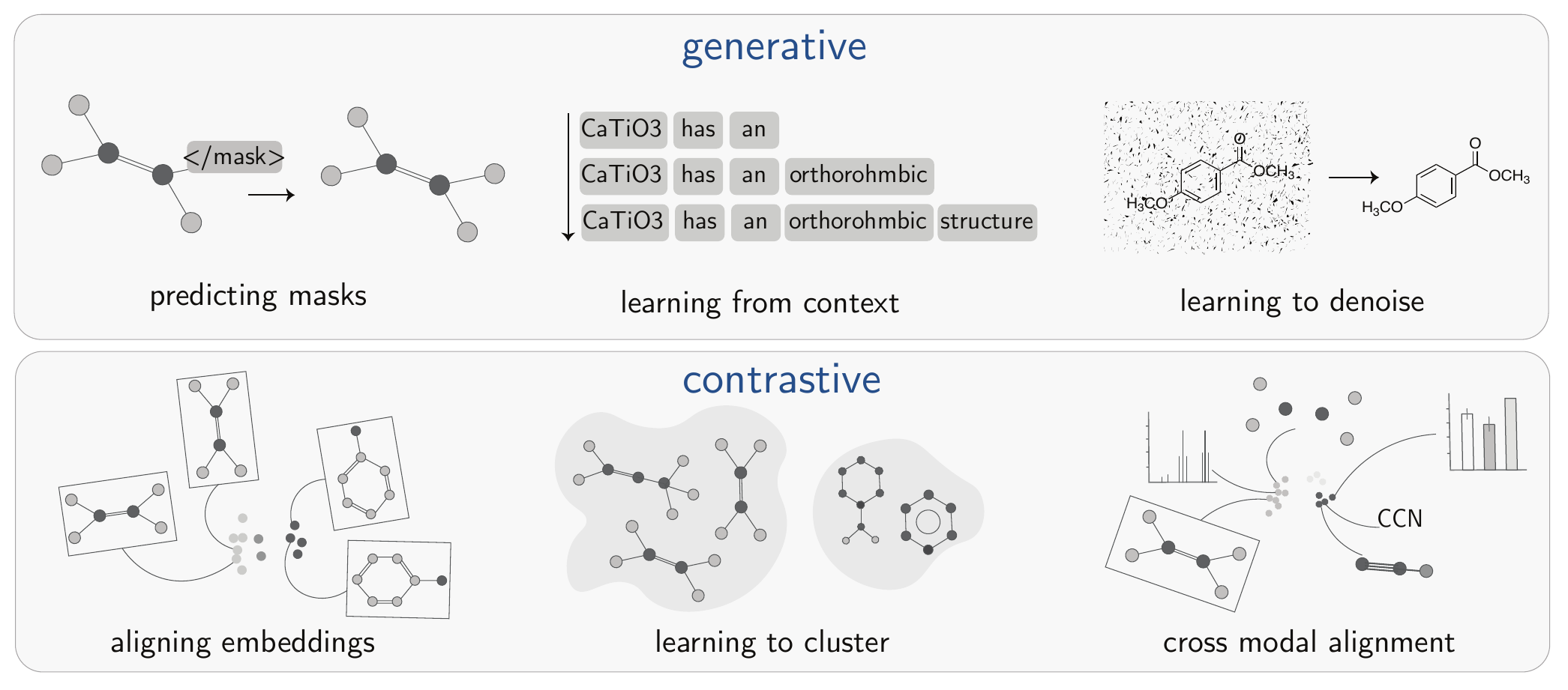
SSL encompasses a variety of approaches. While distinct methods exist, they can be grouped into two main families: generative and contrastive (see Figure 3.2).
3.4.3 Generative Methods
This family of methods focuses on learning representations by reconstructing or predicting parts of the input data from other observed parts. The model learns the underlying data distribution by learning to regenerate the missing information. Examples shown in Figure 3.2 include predicting masked portions of a graph, learning from surrounding text context, and learning to denoise an image.
3.4.3.1 Masked Modeling
In this method, portions of the input data are intentionally obscured or “masked”. The model’s primary objective is then to reconstruct these hidden segments. [Devlin et al. (2018)] This process can be conceptualized as a “fill-in-the-blanks” task, compelling the model to infer missing information from its context. This enables the model to develop a deep understanding of contextual dependencies of data’s structure and semantics without requiring explicit human-labeled annotations. For chemical data, this could involve masking and predicting tokens in or strings [Chithrananda, Grand, and Ramsundar (2020); Zhang et al. (2025)] (i.e., hiding atoms and training the model to guess what is missing), omitting atom or bond types in molecular graphs [Mahmood et al. (2021); Yuyang Wang et al. (2022); Reiser et al. (2022)], removing atomic coordinates in 3D structures, or masking sites within a crystal lattice (see Note 3.3).
Original version: 5.64 5.64 5.64 90 90 90 Na+ 0 0 0 Cl- 0.5 0.5 0.5
Masked version: 5.64 5.64 5.64 90 90 90 Na+ 0 0 0 Cl- <mask>
The model must predict what goes in <mask>, a process that may be informed by the following learned rules and contextual clues.
Context clues: The equal cell lengths and 90 ° angles indicate a cubic symmetry (common for rock salt).
Chemical Knowledge: In ionic crystals like NaCl, cations and anions alternate for charge balance; Cl- typically occupies octahedral sites offset by half the cell in all directions to minimize repulsion.
Correct prediction:
0.5 0.5 0.5(placing Cl- at the cube’s center for proper packing).
This forces the model to understand local ionic coordination (e.g., Na+ surrounded by 6 Cl-) and global crystal architecture.
3.4.3.2 Next Token Prediction
One of the most powerful SSL tasks for sequential data, such as text, is next-token prediction. Here, the core objective is for a model to generate the subsequent token in a given sequence, based on the contextual information provided by preceding tokens. Because text unfolds naturally in a sequence, it offers the reference information the model needs to learn. This approach has been applied to chemical and material representations by treating molecular string representations (SMILESs, SELFIESs, etc.) or material representations as sequences [Adilov (2021); Ye Wang et al. (2023); Schwaller et al. (2019); Alampara, Miret, and Jablonka (2024)]. During training, the model optimization procedure constantly adjusts the model to maximize the likelihood (trying to make good predictions more probable and bad predictions less probable). This is accomplished by making each prediction based on the preceding input, which establishes the conditional context (see Note 3.4).

Prediction Term (Blue): The target token \(x_t\) that the model is trying to predict at each position.
Context Tokens (Maroon): The set of tokens \(x_{\text{context}}\) the model uses to make its prediction. The definition of this context depends on the SSL task:
For Masked Modeling: The context is all unmasked tokens in the sequence.
For Next-Token Prediction: The context is the preceding tokens (\(x_{<t}\)).
Summation \(\sum_{t=1}^{T}\): The loss is calculated across all token positions in the sequence of length \(T\).
The Logarithm’s Role: The negative logarithm (\(\log P\)) heavily penalizes highly confident wrong answers (low \(P\), high loss) and lightly rewards confident correct answers (high \(P\), low loss).
Overall Loss Structure: Cross-entropy loss that encourages the model to assign high probability to the correct next token at each position, given all previous tokens.
3.4.3.3 Denoising
Denoising SSLs works by intentionally adding noise to the inputs and then training models to reconstruct the original data. In this context, the original, uncorrupted data implicitly serves as the label or target for the training process. In this paradigm, we begin with a clean input, which we can call \(x\). We then apply a random corruption process to create a noisy version, \(\tilde{x}\). The model is then trained to reverse the corruption process and recover the original \(x\). This process is formally expressed as sampling a corrupted input \(\tilde{x}\) and optimizing the network to predict \(x\). [Vincent et al. (2010)] By learning to recover the input, the model is compelled to develop robust representations that are inherently invariant to the types of noise it encounters during training. This directly forces the model to learn the underlying data distribution. To distinguish the original signal from the artificial noise, the model must learn the features of high-probability samples within that distribution. For example, to successfully “denoise” a molecule, it must implicitly understand the rules of chemical plausibility that separate valid structures from random noise. Denoising objectives are popular in images [Vincent et al. (2008); Bengio et al. (2013)] and have consequently been applied to graph representations of molecules [Yuyang Wang et al. (2023); Ni et al. (2024)]. For instance, one can randomly perturb atoms or edges in a molecular graph and train a graph neural network to predict the original attributes.
3.4.4 Contrastive Learning
The other main family of SSL techniques is contrastive learning. The objective is to train models to understand data by distinguishing between similar and dissimilar samples. This is achieved by learning an embedding space where representations of samples that are alike in their core chemical properties or identity are pulled closer together. In contrast, representations of samples that are fundamentally different are pushed further apart. [Hadsell, Chopra, and LeCun (2006)]
This process creates meaningful clusters for related concepts while enforcing separation between unrelated ones. In effect, the model learns the data’s underlying distribution by defining the distance between its points. The resulting internal representations become highly robust because they are trained for invariance; the model learns to focus on essential, identity-defining features while disregarding irrelevant variations. This process, often referred to as embedding alignment, ensures that the representations capture the core characteristics shared among similar samples (see Note 3.6).
There are many contrastive learning approaches with variations in loss functions. A key design choice in contrastive learning is whether to compute the contrastive loss on an instance basis or a cluster basis.
3.4.4.1 Instance Discrimination
Instance Discrimination is the most dominant paradigm in recent contrastive learning. Each instance (sample) in the dataset is treated as its own distinct class. This is typically achieved using contrastive loss functions like InfoNCE see Note 3.5. [Oord, Li, and Vinyals (2018)] As detailed in Note 3.5, the loss function is formulated as a categorical cross-entropy loss where the task is to classify the positive sample correctly among a set of negatives plus the positive itself.
In materials and chemistry, this can involve aligning the textual representation of a structure with a graphical representation, image, or other visual method to represent a molecule.[Seidl et al. (2023)] The model could also learn from augmentations of a structure, such as being given several valid SMILES strings that all describe the identical molecule.
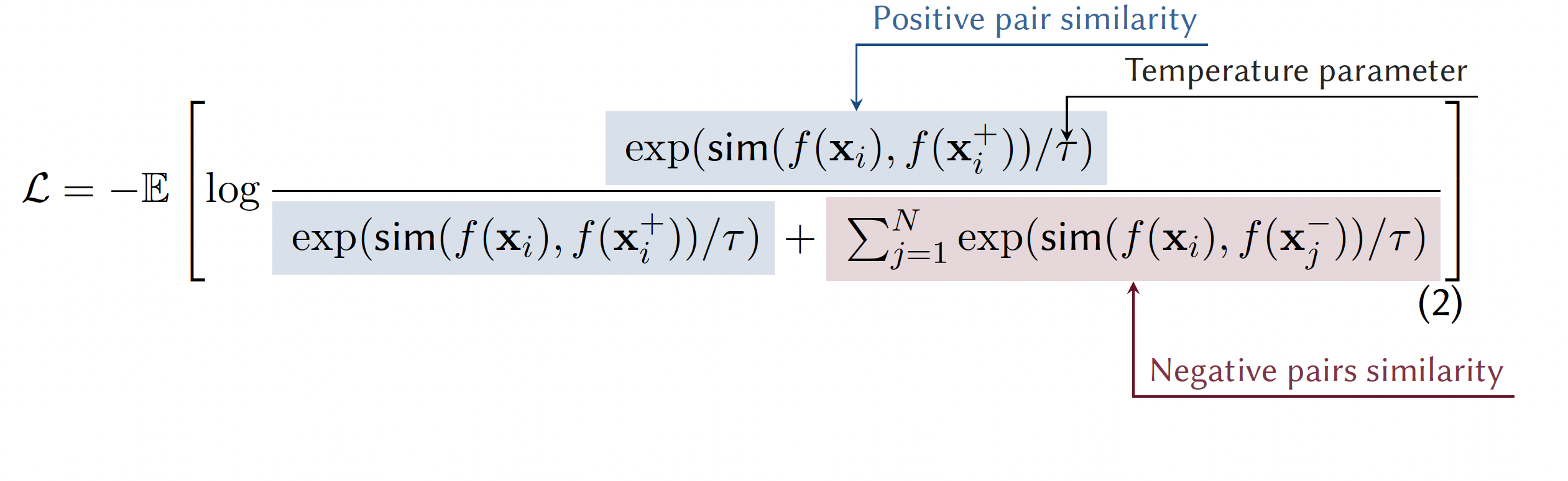
Positive Pair Term (Blue): Measures similarity between an anchor sample \(\mathbf{x}_i\) and its positive pair \(\mathbf{x}_i^+\) (e.g., different view of the same molecule).
Negative Pairs Term (Maroon): Sum of similarities between anchor sample \(\mathbf{x}_i\) and all negative pairs \(\mathbf{x}_j^-\) (e.g., different molecules).
Temperature Parameter \(\boldsymbol{\tau}\) : Controls the sharpness of the distribution. Lower values make the model more sensitive to hard negatives.
Overall Loss Structure : A negative log probability that encourages the model to maximize similarity for positive pairs while minimizing it for negative pairs.
Consider these three molecules:
- Molecule A: Aspirin
(CC(=O)OC1=CC=CC=C1C(=O)O) - Molecule B: Salicylic acid
(OC1=CC=CC=C1C(=O)O) - Molecule C: Glucose
(OC[C@H]1OC(O)[C@H](O)[C@@H](O)[C@@H]1O)
Contrastive learning might:
- Pull A and B together (both contain benzene ring + carboxylic acid)
- Push A and C apart (completely different structures and properties)
- Learn that aromatic compounds cluster separately from sugars
The model learns that structural similarity often correlates with chemical properties.
3.4.4.2 Clustering-based Contrastive Learning
Clustering approaches leverage the idea that similarity often translates to closeness in the feature space. Methods like DeepCluster [Caron et al. (2018)] iteratively train a model. First, they group the generated features (internal representation) of a dataset into distinct sets using a common grouping algorithm, such as \(k\)-means clustering. Imagine you have a pile of diverse objects; \(k\)-means would help you sort them into a predefined number of piles based on their similarities, like color or shape. These assigned groups then act as temporary “pseudo-labels” to train the network. The supervised training step implicitly contrasts samples from different clusters. The clustering and training steps alternate. Take a dataset of molecular fingerprints as an example. A model can be trained to predict the clustering pattern of this fingerprint data, distinguishing between functional group types or structures. Thus, the model learns representations that group chemically or structurally similar fingerprints.
3.5 Building Good Internal Representation
The design of effective pretext tasks—such as specific versions of instance discrimination (identifying unique examples) or denoising (recovering original data from corrupted versions) is where deep domain expertise becomes invaluable.
The pretext tasks must be meaningful, preserving the core identity of the molecule or material while introducing sufficient diversity to challenge the model and allow it to learn robust invariances.
For instance, a suboptimal technique would be to shuffle all the atoms in the text representation of a molecule. This would destroy the molecule’s chemical meaning, which would hinder the model’s ability to learn chemically meaningful features. Good augmentations enable richer features by providing additional layers of information to learn from, such as generating different low-energy conformers or using non-canonical string representations.
3.5.1 Parallels between Generative and Contrastive Objectives
While it might seem that generative and contrastive SSLs methods optimize different things, their underlying goals can be equivalent. A generative masked language model learns the conditional probability (see Note 3.5), aiming to assign a high probability to the correct masked token by effectively discriminating it from other vocabulary tokens. The InfoNCE loss in contrastive learning can be viewed as a log-loss for a \((K+1)\)-way classification task (see Note 3.5). Here, the model learns to identify the positive pair \(f(x_i^+)\) as matching \(f(x_i)\) from a set including \(f(x_i^+)\) and \(K\) negative features \(f(x_j^-)\). Both approaches effectively learn to select the “correct” item (a token or a positive feature) from a set of candidates based on the provided context or an anchor. To do so, they must effectively build strong internal representations.
3.5.1.1 Pre-training beyond SSL
Pre-training be performed using SSL on multiple modalities. For example, in models that consider multiple input formats (multimodality, as explained in detail in Section 3.9.1), alignments between different modalities (e.g., text-image, text-graph) serve as a pre-training step.[Weng (n.d.); Girdhar et al. (2023)] General-purpose force fields are commonly trained in a supervised manner on relaxation and simulation trajectories.[Batatia et al. (2022); Wood et al. (2025)] Thus, the model learns a representation of connectivity patterns to energies. However, these representations also implicitly encode structural patterns (commonly observed coordination environments) and their correlations with each other and with abstract properties. A distinct and powerful pre-training paradigm moves away from real-world data entirely, instead training models like TabPFN on millions of synthetically generated datasets to become general-purpose learning algorithms (see Section 2.3 about dataset creation). This allows them to perform in-context learning on new, small datasets during a single inference call, often outperforming traditional methods. [Hollmann et al. (2025)]
The core principle remains: learning on large datasets to build generalizable internal representations before task-specific fine-tuning.
3.6 Fine-Tuning: Learning the Coloring of Data
While pre-training enables models to learn general structural representations of chemical data, fine-tuning refines these representations for specific downstream tasks. If pre-training can be conceptualized as learning the “structure” of chemical knowledge, fine-tuning can be viewed as learning to “color” this structure with task-specific knowledge and capabilities (see Figure 3.1). This specialization process transforms general-purpose internal representations into powerful task-specific predictors while retaining the foundational knowledge acquired during pre-training.
Fine-tuning adapts pre-trained model parameters through training on domain-specific datasets. This typically requires substantially less data than pre-training. To make this process even more efficient, a common strategy is to “freeze” the majority of the model’s layers and only train a small subset of the final layers (see Section 3.10.3). Fine-tuning is particularly valuable in chemistry, where datasets are often limited in size. Traditionally, addressing chemistry-specific problems required heavily engineered and specialized algorithms that directly incorporated chemical knowledge into model architectures. However, fine-tuned LLMs, for example, have shown comparable or superior performance to these specialized techniques, particularly when data is limited [Jablonka et al. (2024)]. The efficiency of fine-tuning stems from the transferability of chemical knowledge embedded during pre-training, where the model has already learned to spot patterns in molecular structure, reactivity, and chemical terminology sequences.
3.7 Post-Supervised Adaptation: Learning to Align and Shape Behavior
Pre-training and fine-tuning equip the model with a learned distribution, which represents its knowledge about what outputs are plausible or likely. Post-training biases this distribution towards preferred outcomes—such as task-specific goals. The new, desired behavior of the model (called the policy, \(\pi\), in RL) comes from this refined distribution. This shift has a subtle but crucial effect on the internal representations.
Post-training alignment workflows commonly use RL, as the classic loss-minimization approaches—simply fine-tuning on more “correct” examples—can struggle to capture more nuanced, hard-to-label objectives.[Huan et al. (2025)] When the goal is to steer the model toward more intangible qualities, formulating loss functions and collecting a pre-labeled dataset become very challenging. In RL-based alignment, the model is treated as an agent that takes actions (generates text in the case of an LLM) in a trial-and-error environment and receives a reward signal based on the actions it chooses. The RL objective is to maximize this reward by changing the model’s behavior. In the case of LLM, this means compelling it to generate text with the preferred properties. This process transforms the model into a goal-oriented one, where the goal can be to generate stable molecules, solve tasks step-by-step, or utilize tools, depending on the reward function.
During alignment, the foundational embeddings for basic concepts (e.g., a carbon atom) learned during pre-training remain largely intact. This initial state is critical; without a robust, pre-trained LLM, the RL process would be forced to blindly explore an intractably vast space, making it highly unlikely to discover preferred sequences (that it could then reinforce).
The mapping from an input to its final representation is adjusted to become “reward-aware”. For example, the representation of a molecule might now encode not just its chemical structure, but also its potential to become a high-reward final molecule (stable and soluble molecule) [Narayanan et al. (2025)].
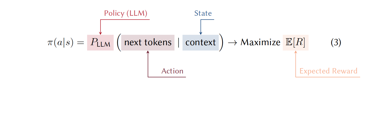
State (s) (Blue): The sequence of tokens generated so far, including the original prompt and any partial response. Represents the current context that the model uses to make decisions.
Action (a) (Maroon): The next token that the model chooses to generate from its vocabulary. This is the discrete decision the agent makes at each step.
Policy (π or PLLM) (Red): The LLM itself, whose parameters define the probability distribution over possible following tokens given the current state. This is what gets optimized during training.
Reward (R) (Peach): A numerical score assigned to complete generated sequences, measuring how well the output achieves the desired goal. Used only during training to guide parameter updates.
Expectation (Eτ∼πθ [R(τ)]) (Peach): The average reward, calculated over many possible sequences τ generated by policy πθ. The subscript τ ∼ πθ indicates that the expectation is taken over the distribution of sequences produced by the current policy. Training adjusts θ to maximize this expectation, enabling the generation of high-quality outputs.
3.7.1 The Challenge of Reward Design
A critical factor for the success of this framework is the design of the reward function. The training process is most stable and effective when rewards are verifiable and based on objective, computable metrics. In contrast, training with sparse rewards (where feedback is infrequent) or fuzzy signals (where the goal is subjective or ill-defined) makes the credit assignment problem significantly more difficult. This is a central challenge in aligning models with complex human preferences, as crafting precise reward functions that capture the full nuance of a desired behavior remains an active area of research [Ouyang et al. (2022)].
3.7.1.1 The LLM as a Policy
When using a LLM as the agent in RL, the policy (see Note 3.7) is the LLM itself. Consider teaching a model to design multi-step synthetic routes for pharmaceutical compounds, using a retrosynthetic strategy. The state (\(s\)) represents the synthetic plan generated so far. Initially, the state consists of just the target molecule but evolves to include each proposed step in the route. Each action (\(a\)) is the next retrosynthetic decision—for example, which bonds to break or what reagents to use. The LLM serves as the policy (\(\pi\)), using its parameters to determine the probability of choosing different possible actions given the current context. To put it mathematically, this would be \(\pi(a|s) = P_{\text{LLM}}(\text{next synthetic step}|\text{current plan})\) (see Note 3.7). The model leverages its chemical knowledge to identify the most promising decisions. The reward (\(R\)) scores the completed retrosynthetic route based on practical criteria that could be the number of steps, predicted yield, reagent cost, etc. This score can directly come from the feedback of real chemists (reinforcement learning from human feedback (RLHF)), or from a small model trained to predict human preference scores or pre-defined criteria (see another example Note 3.8 of optimizing solar cells with RL ).
Theoretical work in reinforcement learning has shown that the complexity of such problems scales quadratically with the size of the action space [Dann and Brunskill (2015)]. At each step, the model must choose from tens of thousands of possible tokens, and the number of possible sequences (and therefore actions) grows exponentially. Without pre-training, this would make the learning process computationally prohibitive. Pre-training provides a strong initialization that effectively constrains the action space to reasonable chemical language and valid synthetic steps, dramatically reducing the exploration requirements (see how pre-training creates a structured manifold in Figure 3.1).
Recent developments have revealed that RL training can elicit reasoning capabilities that were previously thought to require explicit programming or extensive domain-specific architectures. Models trained with RL demonstrate the ability to decompose complex problems, perform backtracking when approaches fail, and engage in multi-step planning without being explicitly taught these strategies. [F. Xu et al. (2025)]
Goal: Design perovskites that are both stable (high thermal/phase stability) and high-performing (optimal bandgap for light absorption).
State: Current partial perovskite formula (e.g., ABX3 lattice with partial cation/anion substitutions).
Action: Substitute the next ion or additive (e.g., replace A-site with Cs+ or add Cl- dopant).
Reward:
+1for stability (e.g., based on Goldschmidt tolerance factor).+1for bandgap tuning (1.5 to 1.8 eVideal for single-junction cells).-1for defect proneness (e.g., halide migration).
Episode Example:
- Start with PbI2 scaffold (B and X sites) \(\rightarrow\) add MA+ (methylammonium) at A-site \(\rightarrow\) Reward:
+0.5(good initial bandgap but low stability due to organic volatility). - Co-substitute with Cs+ and FA+ (formamidinium) \(\rightarrow\) Reward:
+1.7(improved tolerance factor >0.9, stable mixed-cation perovskite with approx.1.6 eVbandgap). - Over-dope with excess Br- \(\rightarrow\) Reward:
-0.7(widens bandgap too much >1.8 eV, reducing PCE; also increases defects).
The model learns to generate perovskite compositions that maximize cumulative reward, naturally discovering stable, high-PCE materials in the vast compositional space for next-gen solar cells. Note, however, that attempting this or a problem would require designing reward functions that can score actions taken by the agent.
3.7.1.2 Updating the LLM Policy
After the model takes actions (generates a sequence of tokens), the reward it receives for the chosen actions is used to update the LLMs parameters using an RL algorithm, such as proximal policy optimization (PPO) [Schulman et al. (2017)]. PPO works by encouraging the model to favor actions (outputs) that lead to higher rewards, but it also includes a mechanism to constrain how much the model’s behavior can change in a single update by introducing s a penalty term that discourages the LLMs policy from deviating too far from its original, pre-trained distribution. This ensures the model does not “forget” its foundational knowledge about language or chemistry while it is learning to pursue the reward, thus biasing the distribution rather than completely overwriting it. The result is a controlled shift: the model becomes more aligned without losing what it already knows.
3.7.1.3 Inference and Sampling from the Adapted Model
The RL training process permanently updates the weights of the LLM. When we sample from this model, we are drawing from this new, biased distribution. For a given context (state), the probabilities for tokens (actions) that were historically part of high-reward sequences are now intrinsically higher. At the same time, pathways that led to low rewards are suppressed. The model is now inherently more likely to generate outputs that align with the preferences and goals encoded in the reward function.
3.8 Example Architectures
While much effort is currently invested in building foundation models based on transformer-based LLMs, the foundation model paradigm is not limited to this model class.
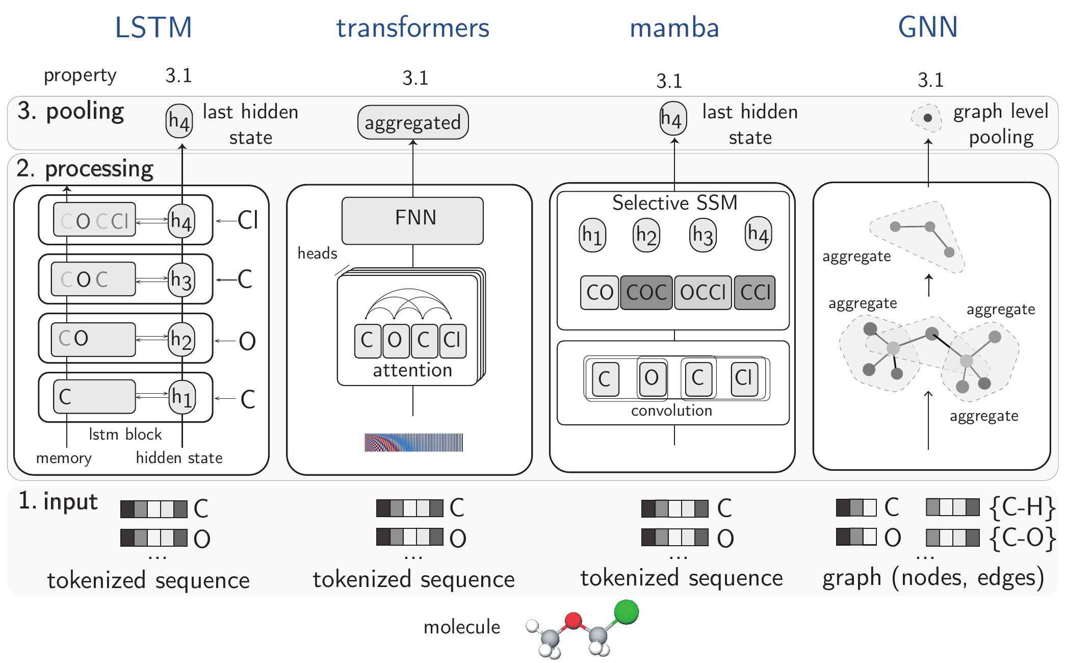
In the chemical domain, where heterogeneous data such as SMILES and graphs for molecular structures prevail, the use of a diverse array of architectures is expected. The architectures shown in Figure 3.3 are examples of foundational backbones that we discuss in the following sections.
3.8.1 LSTM
LSTM networks [Hochreiter and Schmidhuber (1997)] are well-suited for processing sequential data, such as text or time series. Figure 3.3 illustrates how chemical information is processed to predictions in LSTMs.
Input: Molecules are represented as tokenized sequences (e.g., SMILES strings like “COCCl”), processed one token at a time. Each token corresponds to an atom.
Processing: Information flows sequentially through LSTM blocks where each hidden state (\(h_{1}\), \(h_{2}\), \(h_{3}\), \(h_{4}\)) accumulates information about the molecule. The memory cell maintains chemical context through gating mechanisms. The inductive bias is sequential processing—assuming chemical properties emerge from analyzing tokens in order.
Pooling: The final hidden state (\(h_{4}\)) captures the entire molecular information after processing the complete sequence. This last state serves as the molecular representation for the downstream task.
LSTMs process information in a strict sequence. For the model to connect the first word to the last, that information must pass through every single step in between. The computational cost of “talking” across the sequence grows with the sequence length. Furthermore, the entire history of the sequence must be compressed into a single, fixed-size hidden state.
An extended long short-term memory (xLSTM) overcomes this with two key changes. xLSTM uses enhanced gates (act like filters to control what information flows) to precisely revise its memory. Second, instead of a single memory bottleneck, it uses a parallel “matrix memory”. This provides multiple “slots” to store different pieces of information at the same time. This structure allows it to process information in parallel, making it much more efficient. Bio-xLSTM adapts this architecture for biological and chemical sequences, demonstrating proficiency in generative tasks and in-context learning for DNA, proteins, and small molecules.[Schmidinger et al. (2025)]
3.8.1.1 Transformer
Transformers [Vaswani et al. (2017)] are also designed for sequential data, but are particularly powerful in capturing long-range dependencies and rich contextual relationships within sequences. Their core “attention mechanism” allows them to weigh the importance of different parts of the input simultaneously (quadratic computational scaling—if you double the length of the sequence, the amount of work the model needs to do quadruples). Effectively, they can be thought of as a fully connected graph model,[Veličković (2023); Joshi (2025)] where each representation of a token is connected to every other token and can impact its representation.
Input: Similar to LSTMs, data is tokenized and often enhanced with positional encodings (see Figure 3.3, the tokenized sequence is added with positional information, e.g., using a sinusoidal signal—the red-blue spectrum) to maintain information about where in a sequence a token is placed (the attention mechanism itself does not preserve sequence order information).
Processing: Uses attention mechanisms, where every atom/token attends to every other token simultaneously. This enables the capture of long-range interactions between distant elements of the sequence, regardless of their sequential distance. The feed-forward neural network (FNN) transforms these attention-weighted representations. To get a more robust and comprehensive understanding of the relationships within a sequence, models don’t just rely on a single way of “paying attention”. Instead, they employ multiple independent “attention heads” known as multi-head attention.
Pooling: Uses an aggregated representation or special token that combines information from all tokens, enabling global molecular property prediction.
3.8.1.2 Mamba
Mamba[Gu and Dao (2023)] is designed to be highly efficient (linear computational scaling with respect to sequence length) and effective at modeling very long sequences, offering a potentially more scalable alternative to Transformers for certain sequential tasks (for example, modelling very long protein sequences or polymer chains, while retaining strong performance in capturing dependencies.)
Input: Sequences similar to LSTM.
Processing: First applies convolution to capture local contexts, creating representations that incorporate neighboring information. These contextualized tokens are then processed through a selective state space model (SSM). An SSM is a type of sequence model that efficiently captures and summarizes long-range dependencies by tracking an evolving internal “state” (evolving representation of all the relevant information) based on inputs. This SSM dynamically focuses on relevant parts. The inductive bias combines local patterns (through convolution) with efficient selective attention for handling long-range dependencies.
Pooling: Uses the final hidden state (\(h_{4}\)) similar to LSTM, but this state contains selectively processed information that more efficiently captures important features.
This architectural approach has been successfully applied to chemical foundation models, demonstrating state-of-the-art (SOTA) results in tasks like molecular property prediction and generation while maintaining fast inference on a large dataset of SMILES samples.[Soares, Vital Brazil, et al. (2025)]
3.8.1.3 GNN
GNN is an architecture that complements graph representations (see the section discussing graph-based representation Section 3.2.1). Molecules are represented as graphs. GNNs then operate on them by processing node and edge representations. Based on how the nodes are connected through edges, the information in these representations is updated multiple times. This procedure is called message passing (see Figure 3.3). Information from neighbors is aggregated, and this aggregation occurs for all nodes and sometimes also for edges.
Input: Graphs, which are collections of nodes (e.g., atoms) and edges (e.g., bonds).
Processing: Uses message passing through multiple aggregation steps (message would be the information in node or edge at the current stage, and aggregation can be different types of operations like adding information, taking mean, etc, depending on the architecture choice). Each node updates its representation based on messages from its bonded neighbors. The inductive bias is the graph structure itself, which naturally aligns with chemical bonding patterns.
Pooling: Graph-level pooling (e.g., taking the mean of all node representations) aggregates information from all atoms and bonds to create a unified molecular representation, respecting the molecular graph structure.
These architectures cannot solve all problems equally well because they are tailored to different data structures. LSTM and Mamba inherently excel at processing sequential data; Transformers are powerful at capturing global relationships across the entire input, whereas GNNs are designed for graph-structured information. Forcing one type to handle data optimally it was not intended for, often leads to suboptimal performance, inefficiency, or requires extensive, task-specific adaptations that dilute its “general-purpose” nature.[Alampara, Miret, and Jablonka (2024)]
3.9 Multimodality
Multimodal capabilities enable systems to process and understand multiple types of data simultaneously. Unlike traditional unimodal models, which work with a single data type (e.g., text-only or image-only), multimodal models can integrate and reason across different modalities, such as text, images, molecular structures, and spectroscopic data.
The core principle behind multimodal models lies in learning shared representations across different data types. The challenge of creating this shared representation can be addressed through several architectural strategies, each with a different approach to learning the joint distribution of multimodal data. One dominant strategy is joint embedding alignment, where separate, specialized encoders are used for each modality (e.g., a GNN for molecular structures and a Transformer for text). These encoders independently map their respective inputs into their own high-dimensional vector spaces. The key learning objective, often driven by contrastive learning (see Section 3.4.4), is to align these separate spaces.
Another common approach is input-level fusion, where different data types are tokenized into a common format and fed into a single, unified architecture. For instance, a molecular structure might be converted into a SMILES string, an image into a sequence of patches, and text into its standard tokens. These disparate token sequences are then concatenated and processed by a single large model, typically a Transformer.[J. Xu et al. (2025)] The model’s attention mechanism can learn correlations between modalities, e.g., an image patch can “attend” to a word in the description. A more recent and highly efficient variant is adapter-based integration, where a powerful, pre-trained unimodal model (models that take a single type of representation) (like an LLM) is frozen, and a small “adapter network” (see discussion about adapter in Section 3.11) is trained to project the embeddings from a secondary modality (e.g., a molecule) into the LLM’s existing latent space.[S. Liu et al. (2023)] This adapter effectively learns to translate the new data type into the LLM’s native “language”, leveraging the LLM’s vast pre-existing knowledge without the need for complete re-training. For instance, a model might learn that the textual description “benzene ring” corresponds to a specific visual pattern in molecular diagrams and produces characteristic peaks in NMR spectroscopy. This cross-modal understanding enables more comprehensive and contextually rich analysis than any single modality alone could provide.
3.9.1 Multimodal Integration in Chemistry
A molecule’s SMILES string alone might not reveal its 3D conformational preferences. A spectrum alone could suggest many molecular structures. However, coupling these modalities with textual knowledge (e.g., “the sample was prepared by X method”) could narrow down possibilities. Multimodal models have the potential to emulate a human expert who simultaneously considers spectral patterns, chemical rules, and prior knowledge to deduce a structure (see an Note 3.9 of leveraging multimodal data for identifying the chemical). Another motivation is to create generalist artificial intelligence (AI) models. Instead of having multiple independent models—one for spectral analysis, another for molecule property prediction, and another for text mining—a single model could handle diverse tasks by understanding multiple data types. In this way, a researcher can ask a question in natural language, provide a molecule (in the form of a structure file or image) as context, and receive a helpful answer that leverages both structural and textual knowledge.
A chemist finds an unknown white powder in a food sample that is highly soluble in water and tastes sweet. Chemist wants to identify it:
Input Modalities:
- \(^{13}\)C-NMR spectrum: Shows peaks in the 60–100 ppm region, characteristic of carbons bonded to oxygen.
- \(^{1}\)H-NMR spectrum: Multiple peaks in the 3–5 ppm region with complex splitting patterns, indicating protons on oxygen-bearing carbons.
- IR spectrum: Broad, intense peak at 3000–3500 cm\(^{-1}\) (O-H stretching), peaks around 2900 cm\(^{-1}\) (C-H stretching), strong peaks at 1000–1150 cm\(^{-1}\) (C-O stretching, ether and alcohol).
- Mass spectrometry: Molecular ion peak at
m/z = 180. - Text description: “White crystalline solid, sweet taste, highly soluble in water, found in food sample”.
Multimodal Model Reasoning:
- MS + IR \(\rightarrow\) Molecular formula C6H12O6 with multiple hydroxyl groups (polyol).
- NMR \(\rightarrow\) Chemical shifts and splitting patterns consistent with a cyclic structure containing multiple oxygen-bearing carbons; presence of anomeric signals suggests equilibrium between ring forms.
- Text + Chemical Knowledge \(\rightarrow\) Sweet taste and high water solubility point to a simple sugar (monosaccharide).
Based on the evidence, the model hypothesizes the molecule to be D-glucose. Single modality would be insufficient—mass spectrometry alone could match any hexose isomer (fructose, galactose, etc.), but combining spectroscopic fingerprints with physical properties enables confident identification.
MolT5 [Edwards et al. (2022)] adapted the T5 transformer for chemical language by training on scientific text and SMILES strings, using a masking objective to reconstruct masked segments. This approach treats SMILES as a “language”, enabling MolT5 to generate both valid molecules and fluent text. Similarly, Galactica [Taylor et al. (2022)], an LLM, also incorporated SMILES into its training. Later, the MolXPT[Zequn Liu et al. (2023)] model used “paired” examples (SMILES and textual description) by replacing chemical names in scientific texts with their corresponding SMILES strings and description. This pre-training approach enables MolXPT to learn the context of molecules within text and achieve zero-shot text-to-molecule generation (see Section 6.2 for more details on this application).
Contrastive learning emerged as an alternative, aligning separate text and molecule encoders in a shared embedding space (see Section 3.4.4 for the principle of learning). MoleculeSTM [S. Liu et al. (2023)] aligns separate text and molecule encoders in a shared space using paired data. This dual-encoder approach enables tasks such as retrieving molecules from text queries and shows strong zero-shot generalization for chemical concepts. CLOOME [Sanchez-Fernandez et al. (2023)] used contrastive learning to embed bioimaging data (microscopy images of cell assays) and chemical structures of small molecules into a shared space. Multimodal learning also enables the determination of molecular structure from spectroscopic data. Models trained on large datasets of simulated spectra [Alberts et al. (2024)], which combine multiple spectral inputs, could accurately translate spectra into molecular structures. [Chacko et al. (2024); A. Mirza and Jablonka (2024)]
Beyond prediction, some multimodal models aim for cross-modal generation, creating one type of data from another (e.g., generating an IR spectrum from a molecular structure). Takeda et al. (2023) developed a multimodal foundation model for materials design, integrating SELFIES strings, density functional theory (DFT) properties, and optical absorption spectra. Their approach involves encoding each type of data separately into a shared, compressed representation space. Then, a network learns to combine these compressed representations to understand the connections between them. This pre-training on a big dataset of samples enables both combined representations (joint embeddings summarizing all modalities) and cross-modal generation, allowing tasks like predicting a spectrum from a molecule or generating a molecule from desired properties. However, inverse generation remains challenging with lower accuracy than forward prediction, generated outputs often require experimental validation, and performance degrades for out-of-distribution molecules.
A more recent approach is the integration of molecular encoders with pre-trained LLMs. Models like InstructMol [Cao et al. (2023)] and ChemVLM [Li et al. (2024)] use an “adapter” (see discussion about LoRa in Section 3.11) to project molecular information into the LLM’s existing knowledge space. This two-stage process first projects molecule representations into the LLM’s token space through pre-training on molecule-description pairs. Subsequently, instruction tuning on diverse chemistry tasks (e.g., questions & answers (Q&A), reaction reasoning) enables the LLM to leverage molecular inputs, significantly enhancing its performance on chemistry-specific problems.
The latest generation of GPMs is often natively multimodal, designed from the ground up to process text, images, and other data types seamlessly. Natively multimodal systems are characterized by a single, unified neural network trained end-to-end on a diverse range of data modalities. In the scientific domain, natively multimodal systems are still being explored. However, evaluations suggest that these models are not yet robust for solving complex scientific research tasks.[Alampara et al. (2025)]
3.10 Optimizations
As GPMs continue to grow in size and complexity, optimization techniques (performance or resource consumptions optimization) become critical for making these models practically deployable while maintaining their accuracy. This section discusses three key optimization approaches that have particular promise for chemistry foundation models: mixture of experts (MoE) architectures for efficient scaling, quantization, and mixed precision for memory and computational efficiency, and knowledge distillation for creating specialized, lightweight models.
3.10.1 Mixture-of-Experts
MoE is a neural network architecture that uses multiple specialized “expert” networks instead of one single, monolithic model. The core idea is to divide the vast problem space—the embedding space of all possible inputs—into more manageable, homogeneous regions. A region is considered “homogeneous” not because all inputs within it are identical, but because they share similar characteristics and can be processed using a consistent set of rules. For instance, in a chemistry model, one expert might specialize in organic molecules, while another focuses on inorganic crystals; each expert sees a more consistent, or homogeneous, set of problems. This division of labor is managed by a gating network, which acts like a smart dispatcher. This gating network is itself a small neural network, often referred to as a trainable router, because it learns during training how best to route the data to the most appropriate expert, thereby improving its decisions over time. MoE models achieve efficiency through selectively activating only the specific experts needed for a given task, rather than activating the entire neural network for every task. Modern transformer models using MoE layers can scale to billions of parameters while maintaining manageable computational costs, as demonstrated by models like Mixtral-8x7B[Jiang et al. (2024)], which uses eight experts with sparsity.
Shazeer et al. (2017) demonstrated that using a sparsely-gated MoE layer can expand a network’s capacity (by over 1000 times) with only minor increases in computation. In this architecture, each expert is typically a FNN, and a trainable router determines which tokens are sent to which experts, allowing only a subset of the total parameters to be active for any given input.
An LLM for science with MoE architecture (SciDFM [Sun et al. (2024)]) shows that the results of expert selection vary with data from different disciplines, i.e., activating distinct experts for chemistry vs. other disciplines. They consist of multiple “expert” subnetworks, each potentially specializing in different facets of chemical knowledge or types of chemical tasks. A routing mechanism directs inputs to the most relevant expert(s). This allows the foundation model to be more adaptable and perform across the broad chemical landscape.
Extending this concept, a recent multi-view MoE model (Mol-MVMoE [Soares, Shirasuna, et al. (2025)]) treats entire, distinct chemical models as individual “experts”. Rather than routing tokens within one large model, a gating network learns to create a combined molecular representation by dynamically weighting the embeddings from each expert model. This method showed strong performance on MoleculeNet, a widely used benchmark suite for molecular property prediction, outperforming competitors on 9 of 11 tasks.
Training MoE models can be a complex process. The gating mechanism must be carefully learned to balance expert usage and instability, or some experts may end up underutilized (most of the data would be processed by a subset of networks). (Fedus, Zoph, and Shazeer 2022) For chemistry tasks, an additional challenge is to ensure that each expert has access to sufficient relevant chemical data to specialize. If the data is sparse, some experts may not learn meaningful functions. Despite these hurdles, MoE remains a promising optimization strategy to handle the breadth of chemical space.
3.10.2 Quantization and Mixed Precision
Quantization is a technique for making models more computationally efficient by reducing their numerical precision. In experimental science, precision often relates to the number of significant figures in a measurement; a highly precise value, such as \(3.14159\), carries more information than a rounded one, like \(3.14\). Similarly, a model’s knowledge is stored in its weights, which are organized into large matrices of numbers. Standard models typically use high-precision formats, such as 32-bit floating-point, which can represent a wide range of numbers with many decimal places to store weights. During inference, these weight matrices are multiplied by the input data to produce a prediction. Quantization involves converting these numbers into a lower-precision format, such as 8-bit integers, which are whole numbers with a much smaller range. This process is similar to rounding experimental data—it simplifies the numbers, uses less memory, and allows calculations to run much faster.
Dettmers et al. (2022) introduced an 8-bit inference approach (LLM.int8) enabling models as large as GPT-3 (175B parameters) to run with no loss in predictive performance (less than \(50\%\) GPU-memory usage). A key insight in this paper is that while most numbers in a model can be safely rounded, a few “outlier” values with large magnitudes are critical for performance.
A different, yet related, strategy is mixed-precision quantization.[Micikevicius et al. (2017)] Instead of applying a single precision format (like 8-bit) across the entire model, this approach uses a mix of different precisions for different parts of the network. The guiding principle is that some layers of the model might be more sensitive to rounding errors than others.
Many chemistry applications, particularly in automated laboratory setups, require deployment on edge devices—local computing hardware, such as the controllers for robotic arms or the onboard computers in analytical instruments—or cloud platforms with limited computational resources. Quantization can be a valuable optimization tool for reducing computational burden while increasing inference speed, which is crucial for real-time applications.
3.10.3 Parameter-Efficient Tuning
While full fine-tuning is computationally expensive, memory-intensive, and results in a complete, multi-gigabyte copy of the model for every new task. parameter-efficient fine-tuning (PEFT) methods offer a solution to this problem by freezing the vast majority of the trained model’s weights and only training a few new parameters.
A prominent and widely used PEFT technique is low-rank adaptation (LoRA).[Hu et al. (2021)] The key insight of LoRA is that the change needed to adapt a pre-trained weight matrix for a new task can be approximated effectively using much smaller matrices. LoRA freezes the original model weights and introduces small trainable rank-decomposition matrices into each transformer layer, significantly reducing the number of trainable parameters. Because these new matrices contain far fewer parameters—often less than 0.1% of the original model—the computational and memory requirements for training are drastically reduced.
These optimization strategies can be combined with quantization (see Section 3.10.2) for even greater efficiency. Dettmers et al. (2023) introduced quantized low-rank adaptation (QLoRA). In this approach, the large pre-trained model is first quantized down to a very low precision (typically 4-bit), dramatically shrinking its memory footprint. Then, the lightweight LoRA adapters are added and fine-tuned. QLoRA enables the fine-tuning of massive models—such as a 70-billion-parameter model—on a single, consumer-grade GPU.
3.10.4 Distillation
Knowledge distillation is a technique that aims to transfer the learning of a large pre-trained model (the “teacher model”) to a smaller “student model”. [Hinton, Vinyals, and Dean (2015)] The computationally more efficient “student model” is trained to mimic the behavior (e.g., output probabilities or internal representations) of the larger teacher model. This allows the rich, nuanced understanding learned by the large foundation model to be compressed into a more compact and faster student model.[Sanh et al. (2019)]
Effective distillation requires that the teacher model is both competent at the task and that its knowledge is representable by the student. If the teacher is too large or complex compared to the student, the student may struggle to emulate it, leading to degraded performance. [Zichang Liu et al. (2024)]
3.11 Model Level Adaptation
Although promising, as shown in Table 3.2, GPMs such as LLMs rarely work straight out of the box for specialized tasks and often need customization. This is especially true for scientific problems where data is a limiting factor. By prompting an LLM—for example, by asking a question or giving instructions—one can observe that these models perform much better on general tasks than on those related to chemistry. This difference arises because LLMs are not typically trained on domain-specific chemical tasks and therefore they lack the necessary knowledge and reasoning skills.
To bridge this gap, two complementary families of approaches exist. The first approach involves adapting the model’s knowledge or behavior directly. The simplest method is to embed information directly in the prompt, for instance by providing examples (in-context learning (ICL)) [Brown et al. (2020)] or by introducing intermediate reasoning steps (chain-of-thought (CoT)) [Wei et al. (2022)]. However, not all problems can be solved in this way, and sometimes it is necessary to tune the model to new data, which updates its parameters. The second approach involves coupling the model into a larger system that can interact with external sources of information and tools.
| Model adaptation | Time | Data | ML knowledge | Energy Cost |
|---|---|---|---|---|
| Pre-training | Weeks | 1M–1B+ | Very High | 50MWh - 1GWh |
| Zero-shot prompting | Minutes | None | None | <10Wh |
| Few-shot Prompting | Hours | <10 | None | <1kWh |
| Fine-tuning | Days | <10k | High | 100kWh - 50MWh |
| Coupling into systems | ||||
| RAG | Days | 100k–1M+ | Low | <1kWh |
| Tool-Augmentation | Days | None / 10k+ | Low | <1kWh |
3.11.1 Prompting
LLMs have demonstrated the ability to perform a wide range of tasks based solely on prompt instructions—without the need for fine-tuning [Radford et al. (n.d.)]. This ability, for LLMs to complete tasks without any additional information, is often referred to as zero-shot prompting. By providing task-specific examples directly within the input prompt, LLMs can draw analogies and generalize to new tasks, a capability known as ICL [Brown et al. (2020); Chowdhery et al. (2023); OpenAI et al. (2023)]. In ICL, the model is presented with a few demonstration examples alongside a query, all within the same input—a technique known as few-shot prompting. The model’s parameters remain unchanged; instead, it is expected that the model can recognize patterns within the prompt and generate an appropriate response [Von Oswald et al. (2023)]. ICL enables models to learn on the fly, reducing the barrier to entry for users without deep ML expertise. However, because the model does not retain memory between queries, the learned knowledge is temporary and is subsequently lost in subsequent queries. Additionally, ICL tends to struggle with tasks that require multi-step reasoning [Brown et al. (2020)]. To address this limitation, task decomposition techniques have been introduced, with the earliest being CoT [Wei et al. (2022)]. Rather than relying solely on examples, this approach enriches the prompt with a series of reasoning steps that guide the model toward the correct answer [Wei et al. (2022)]. Considering that prompting approaches do not require an in-depth understanding of machine learning, they have proven very useful for a range of chemical tasks, including chemical data extraction, Q&A, and property prediction [H. Liu et al. (2025); Zheng et al. (2023); Adrian Mirza et al. (2025); Ramos et al. (2023)].
3.11.1.1 Fine-tuning
Fine-tuning directly changes the weights of the model (see Section 3.6). The fine-tuning strategy depends on the size and complexity of the target dataset as well as the pre-trained model. For many tasks, especially when using a powerful pre-trained model, it is often sufficient to freeze the entire model except for the final layer and only train that layer’s parameters. However, as the target task diverges more significantly from the pre-trained model’s original objectives, more adaptation may be necessary. This can include replacing specific layers in the model to better suit the new task. For instance, in autoencoder architectures, it’s common to freeze the encoder and replace the decoder. In GNNs, the graph convolutional layers are typically frozen, while the final fully connected layers are replaced and re-trained. In some cases, it may be necessary to fine-tune the entire model, an especially resource-intensive process for LLMs, whose parameters can be in billions. Despite these innovations, one key limitation of fine-tuning remains: adapting to a new modality, which often requires architectural changes or switching to a different model. However, LLMs offer a unique workaround. Many regression or classification tasks can be reformulated into a text-based format, allowing a single language model to be fine-tuned across a wide range of tasks. This is known as language-interfaced finetuning (LIFT) [Dinh et al. (2022)], which enables us to utilize a single GPM for a diverse set of tasks.
Beyond adapting a model’s internal knowledge through prompting or fine-tuning, its capabilities can be expanded by coupling it with external resources. This approach transforms a static model into a dynamic problem-solver that can access up-to-date information and perform actions in the world. This practice of designing and delivering task-relevant information is often referred to as context engineering. The necessary context can be provided through several complementary approaches that operate during inference time.
3.12 System-level Integration: Agents
While powerful, GPMs are fundamentally static entities. Their knowledge is frozen at the time of training, and they cannot interact with the world beyond the information they process. They cannot browse the web for the latest research, execute code to perform a calculation, or control a robot to run an experiment. To overcome these limitations and apply the reasoning capabilities of GPMs to complex, multistep scientific problems, so-called LLM-based agents have emerged.
An LLM-based agent is a system that leverages an LLMs as its core “brain” but couples it with a set of tools to perceive and act upon its environment. To use a tool, the agent generates text containing the tool’s name and its required inputs (arguments). The framework managing the agent recognizes this specific text, executes the corresponding tool, and then feeds the result back to the LLM. This transforms the model from a passive generator of text into an active problem-solver that can formulate plans, execute actions, observe the results, and adapt its strategy accordingly. For chemists and material scientists, this paradigm shift is profound. It moves from asking a model a question to giving it a research goal, which it can then pursue autonomously.
Figure 3.4 illustrates the fundamental components of an agentic framework, often conceptualized through the interacting modules of perception, cognition, and execution. It is important to note that this is one possible way to formalize an agent’s architecture; other organizational structures exist. Rather than a strict, sequential loop, these components represent a set of capabilities that the agent’s core LLM can dynamically draw upon to achieve complex objectives.
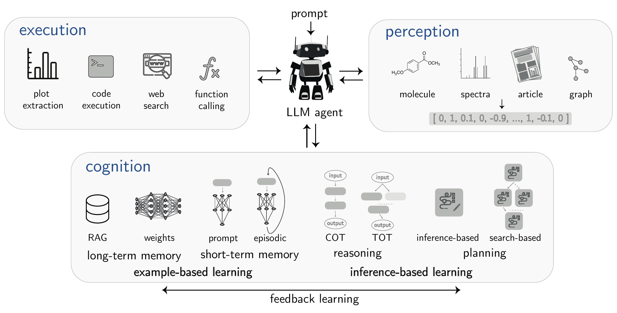
3.12.1 Core Components of an Agentic System
An agent is a system composed of several key components that work in concert.
3.12.1.1 Cognitive Engine
This is typically a powerful LLM, though other approaches exist, including classical planning systems or hybrid systems. Modern implementations may interface with LLMs via internal representations (hidden states) rather than solely through text output.
It is responsible for all high-level reasoning, including understanding the user’s objective, breaking it down into smaller, manageable steps (see Section 5.5), and deciding which tools to use to accomplish each step.
3.12.1.2 Tool Augmentations (Execution)
Tools are external programs or functions that the agent can call upon to perform actions. They allow agents to interact with the world beyond their internal knowledge. [Schick et al. (2023); Parisi, Zhao, and Fiedel (2022)]. Tool augmentation can range from simple tools, such as calculators, to more complex systems that involve web searches, code execution, and integration with robots [Darvish et al. (2025); Chan et al. (2024); Wei et al. (2025)]. In a chemical context, tools can be as simple as a stoichiometry calculator or as complex as a Python script that runs a DFT simulation using specialized software, a search application programming interface (API) for querying chemical databases like PubChem, or a controller for a robotic synthesis platform [Boiko et al. (2023); Darvish et al. (2025); Bran et al. (2024)].
3.12.1.3 Memory & retrieval-augmented generation (RAG)
Agents need to maintain context over long and complex tasks. The memory module provides this capability. Short-term memory is often handled within the finite context window (i.e., number of tokens an LLM can process), keeping track of the immediate chain of thought and recent actions. While short-term memory (e.g., context) is transient, LLMs model weights serve as long-term memory. However, these weights often lead to reduced performance on knowledge-intensive scientific tasks and increased susceptibility to hallucinations—generating incorrect or fabricated information [Marcus (2020)]. One effective way to address this limitation is to pair the model with an external knowledge base.[Lewis et al. (2020)] Such Long-term memory can be implemented using external databases (e.g., vector stores) where the agent can store and retrieve key findings, successful strategies, or experimental results from past interactions, enabling it to learn and improve over time [K. Chen et al. (2023)]. The widely adopted execution of Long-term memory is RAG. RAG works by retrieving a set of relevant documents from a designated knowledge database based on the input query. These retrieved documents are then concatenated with the original prompt and passed to the LLM, which generates the final output. In scientific applications, this is particularly valuable, as the system can be continuously updated with the latest research and discoveries. In the field of chemistry, RAG has primarily been used to answer domain-specific questions based on scientific literature and assist in experimental design [K. Chen et al. (2023); Skarlinski et al. (2024)].
3.12.2 Approaches for Building Agentic Systems
A well-known approach for building LLM-based agents is called reasoning and acting (ReAct)[Yao et al. (2023)]. In ReAct, the agent repeatedly goes through a cycle of thinking, performing an action, and then reasoning about the tool output. This structured problem-solving is achieved by prompting the model to generate its response following a specific “Think”, “Act”, “Observe” format. First, the agent considers the problem it needs to solve, focusing on its primary objective. It devises a plan, identifies any missing information, and determines which tool can help it move forward. Next, the agent acts by selecting and utilizing the appropriate tool with the necessary information. For instance, if it needs to find a compound’s boiling point, it might use a tool that searches a chemical database using the compound’s name or its SMILES string. After that, the agent observes the outcome by examining the tool’s output. This output then becomes new information for the agent. The agent then repeats the cycle, taking this new observation into account as it plans its following action. This loop continues until the agent reaches its main goal (see Note 3.10). This repeating process helps the agent deal with mistakes, adjust to unexpected results, and break down a big task, like “finding a better catalyst for this reaction”, into smaller, manageable steps that involve using tools (see example below).
User Query: “Identify this unknown white solid organic compound from analytical data.”
Agent Reasoning Cycle:
- THINK: “Unknown white solid. Need to analyze all spectra systematically.”
- ACT: Analyze
IRspectrum tool \(\rightarrow\) Output peak data (3000 cm–3500 cm broad, 1680 cm sharp, 1600 cm, 1500 cm). - ACT: Analyze
MStool \(\rightarrow\) Output peak data (Top 3 peaks (135.0, 26.48),(106.9, 0.43),(120.4, 0.31)). - OBSERVE: “Broad
O-Hstretch suggests carboxylic acid. SharpC=Oat1680indicates aromatic carboxylic acid. AromaticC=Cstretches confirm benzene ring, andMStool suggests molecular formula C8H8O2.” - THINK: “Aromatic carboxylic acid with C8H8O2... probably substituted benzoic acid. Need to determine substitution pattern.”
- ACT: Run ^1H
NMRintegration tool \(\rightarrow\) Input chemical shifts (7.8 ppmdoublet,7.3 ppmdoublet,2.4 ppmsinglet,12.1 ppmbroad). - OBSERVE: “Two aromatic doublets suggest para-disubstitution. Singlet at
2.4 ppmintegrates for3H— likely CH3. Broad peak at12.1 ppmconfirms COOH.” - THINK: “Para-disubstituted benzene with CH3 and COOH groups. Could be p-toluic acid.”
- ACT: Search chemical database for “
para-methylbenzoic acid”. - OBSERVE: “
4-methylbenzoic acid(p-toluic acid) matches: C8H8O2,mp180 ° C.” - ACT: Run structure validation tool \(\rightarrow\) Compare predicted vs. observed spectra.
- OBSERVE: “Predicted ^1H
NMR: \(\delta\)7.9 (d, 2H),7.2 (d, 2H),2.4 (s, 3H),12.0 (br, 1H). Perfect match!” - ACT: Cross-reference
MSfragmentation pattern tool. - OBSERVE: “Base peak at
m/z 91(tropylium ion, loss of COOH), molecular ion at136. Consistent with p-toluic acid fragmentation.”
RESULT: Structure confirmed as 4-methylbenzoic acid. All spectroscopic evidence supports this assignment.
The agent systematically combines IR, NMR, and MS data with database searching to solve a realistic structure determination challenge.
Scientific discovery often requires diverse expertise and collaborative problem-solving. This has led to the development of multi-agent systems, which move beyond a single cognitive engine to orchestrate a team of agents that work together [Wu et al. (2023)]. These systems can solve tasks that are too complex or multifaceted for any single agent to handle alone by enabling agents to communicate, delegate, and debate. [Lazaridou and Baroni (2020)] Several collaborative paradigms have emerged, each offering unique advantages:
3.12.2.1 Specialization and Division of Labor
Just as a human research group has members with different roles, multi-agent systems can be composed of specialized agents. For example, in a chemistry context, a “Planner” agent might design a high-level research plan, a “Literature Searcher” agent could retrieve relevant papers, a “Computational Chemist” agent could run DFT simulations, and a “Safety Expert” agent could check proposed reaction steps for hazards.[Zou et al. (2025)] This division of labor shows this role-playing approach to be highly effective for complex tasks like software development, where agents take on roles such as “programmer”, “tester”, and “documenter” [Qian et al. (2024)].
3.12.2.2 Refinement of Answers
A key weakness of single LLMs is their tendency to hallucinate or pursue a flawed line of reasoning. Multi-agent systems can mitigate this by introducing criticism and debate. In this paradigm, one agent might propose a solution (e.g., a synthetic pathway), while a “Critic” agent is tasked with finding flaws in the proposal. This adversarial or collaborative process forces the system to refine its ideas, correct errors, and explore alternatives, leading to more robust and reliable outcomes [Liang et al. (2024); Du et al. (2023)].
3.12.2.3 Context Compression through Parallelism
A significant operational challenge for any LLM-based system is the finite context window. As a task becomes more complex, the conversational history can grow cluttered with irrelevant details, degrading the model’s performance.[Chirkova et al. (2025); Lee et al. (2024)] Multi-agent systems offer a solution to this problem through a strategy that can be described as context compression. By assigning sub-tasks to specialized agents, the system allows each agent to operate in parallel with its own clean, dedicated context window. For example, a “Literature Searcher” agent’s context is filled only with search queries and retrieved text, while a “Computational Chemist” agent’s context contains only simulation inputs and results. These sub-agents essentially act as filters; they process large amounts of information and then “compress” their findings into concise summaries or structured data. These distilled insights are then passed back to a lead agent or aggregated. This not only speeds up information gathering but also ensures that the primary reasoning process is not diluted by excessive or irrelevant information [Breunig (n.d.)].
3.12.2.4 Swarm Intelligence and Parallel Exploration
Inspired by natural systems like ant colonies, some multi-agent approaches use a “swarm” of less-specialized agents to explore a vast problem space in parallel. Instead of assigning fixed roles, a multitude of agents can independently investigate different hypotheses or search different regions of a chemical space. Their collective findings can then be aggregated to identify the most promising solutions. This is particularly powerful for optimization and discovery tasks, such as high-throughput virtual screening or materials design, where the goal is to efficiently search an enormous number of possibilities [W. Chen et al. (2023)].
3.13 Models vs. Systems
It is also crucial to distinguish between the foundational model itself (e.g., the GPT-4 LLM) and the “system” with which the user interacts (e.g., ChatGPT). Such systems are not merely the raw model; they incorporate additional layers for safety, prompt management, and some adaptation techniques discussed in this section.